4Marginal Distributions of Discrete Random Variables
Random variables measure numerical quantities of interest associated with a random phenomenon. Random variables can potentially take many different values, usually with some values or intervals of values more probable than others. Even when outcomes of a random phenomenon are equally likely, values of related random variables are usually not. The (probability) distribution of a collection of random variables identifies the possible values that the random variables can take and a way of determining their relative likelihoods. We will see several ways to describe distributions, some of which depend on the number and types (discrete or continuous) of the random variables under investigation.
Commonly encountered random variables can be classified as discrete or continuous (or a mixture of the two1).
A discrete random variable can take on only countably many isolated points on a number line. These are often counting type variables. Note that “countably many” includes the case of countably infinite, such as \(\{0, 1, 2, \ldots\}\).
A continuous random variable can take any value within some uncountable interval, such as \([0, 1]\), \([0,\infty)\), or \((-\infty, \infty)\). These are often measurement type variables.
We will see a few ways of specifying a distribution, including
A well labeled plot
A table of possible values and corresponding probabilities for discrete random variables. This could be a two-way table for the joint distribution of two discrete random variables (or multi-way table)
A probability mass function for discrete random variables which maps possible values \(x\) — or \((x, y)\) pairs, etc — to their respective probability.
A probability density function for continuous random variables which maps possible values \(x\) — or \((x, y)\) pairs, etc — to their respective probability “density”.
A cumulative distribution function, which provides all the percentiles (a.k.a. quantiles) of the distribution
By name, including values of relevant parameters, e.g., “Uniform(0, 60)”, “Normal(30, 10)”, “Poisson(1)”, “BivariateNormal(30, 30, 10, 10, 0.7)”. We will see that some probabilistic situations are so common that the corresponding distributions have special names. Each named distribution has corresponding parameters, e.g., 0 and 60 are the parameters of the Uniform(0, 60) distribution. Always be sure to specify values of relevant parameters, e.g., “Normal(30, 10) distribution” rather than just “Normal distribution”. Be careful: different named distributions have different identifying parameters. For example, the parameters 0 and 60 mean something different for the Uniform(0, 60) distribution than for the Normal(0, 60) distribution.
Distributions of random variables can be thought of as collections of probabilities of events involving the random variables. As for probabilities, we can interpret probability distributions of random variables as:
long run relative frequency distributions: what pattern of values would emerge if we repeated the random process many times and observed many values of the random variables?
subjective probability distributions: which potential values of these uncertain numerical quantities are relatively more plausible than others?
Regardless of the interpretation, we can use simulation to investigate distributions of random variables: simulate many values of the random variables and summarize them in various ways to describe the pattern of variability. We will often represent distributions as spinners (or a collection of spinners) which when spun many times achieve the appropriate long run pattern of values of the random variables.
Most interesting problems involve two or more random variables defined on the same probability space. In these situations, we can consider how the variables vary together and study relationships between them. A joint distribution describes the full pattern of variability of a collection of random variables. In the context of multiple random variables, the distribution of any one of the random variables alone is called a marginal distribution.
In this chapter we’ll investigate marginal distributions of discrete random variables. We have already been introduced to distributions of discrete random variables; see Section 2.5 and Section 3.5. Now we’ll explore in more detail.
4.1 An introductory example
Example 4.1 Capture-recapture sampling is a technique often used to estimate the size of a population. Suppose you want to estimate \(N\), the number of monarch butterflies in Pismo Beach. (Assume that \(N\) is a fixed but unknown number; the population size doesn’t change over a short time.) You first capture a sample of \(N_1\) butterflies, selected randomly, and tag them and release them. Later you capture a second sample of \(n\) butterflies, selected randomly with replacement. (We’ll compare to the case of sampling without replacement later.) Let \(X\) be the number of butterflies in the second sample that have tags (because they were also caught in the first sample). (Assume that the tagging has no effect on behavior, so that selection in the first sample is independent of selection in the second sample.)
In practice, \(N\) is unknown and the point of capture-recapture sampling is to estimate \(N\). But let’s start with a simpler, but unrealistic, example where there are \(N=52\) butterflies, \(N_1 = 13\) are tagged and \(N_0=52-13 = 39\) are not, and \(n=5\) is the size of the second sample.
What are the possible values of \(X\)?
Describe how you could use a tactile simulation to simulate a single value of \(X\).
Describe in words how you could use simulation to approximate \(\textrm{P}(X=0)\).
Describe in words how you could use simulation to approximate the distribution of \(X\).
Write and run Symbulate code to approximate \(\textrm{P}(X=0)\) and the distribution of \(X\).
Construct a table, plot, and spinner representing the approximate distribution of \(X\).
The theoretical value of \(\textrm{P}(X = 0)\) is 0.237. (We will see how to compute this later.) Compare to your simulated value. Is the theoretical value within the margin of error of the simulated value?
Interpret in context \(\textrm{P}(X = 0) = 0.237\) as a long run relative frequency.
Describe in words the distribution of \(X\). What are some relevant features?
Solution (click to expand)
Solution 4.1.
\(X\) is the number of tagged butterflies in the sample of 5, so the largest \(X\) can be is 5 and the smallest \(X\) can be is 0. (Don’t forget 0.) The possible values of \(X\) are 0, 1, 2, 3, 4, 5.
We could use a deck of 52 cards, with 13 labeled “tagged” (say the clubs) and the others not. Shuffle the deck and draw 5 cards with replacement, and let \(X\) be the number of cards out of the 5 drawn that say “tagged”.
Repeat the steps in part 2 many times to simulate many values of \(X\), say 10000. Count the number of repetitions that result in \(X=0\) and divide by the total number of repetitions (10000); this relative frequency approximates \(\textrm{P}(X = 0)\).
Simulate many values of \(X\) (say 10000) and find the simulated relative frequency of each possible value: \(0, 1, 2, 3, 4, 5\).
See Symbulate code below.
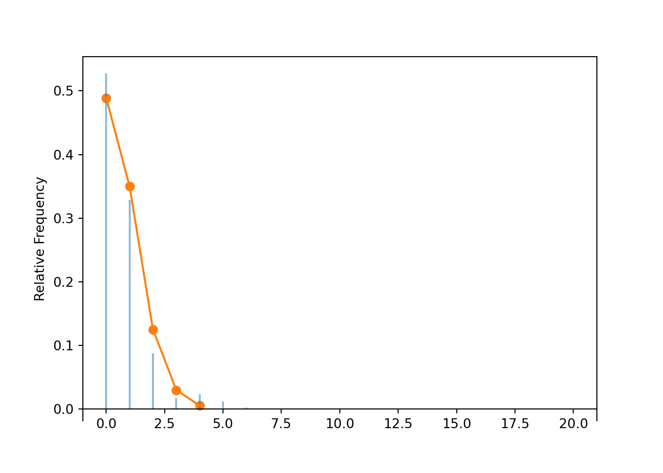
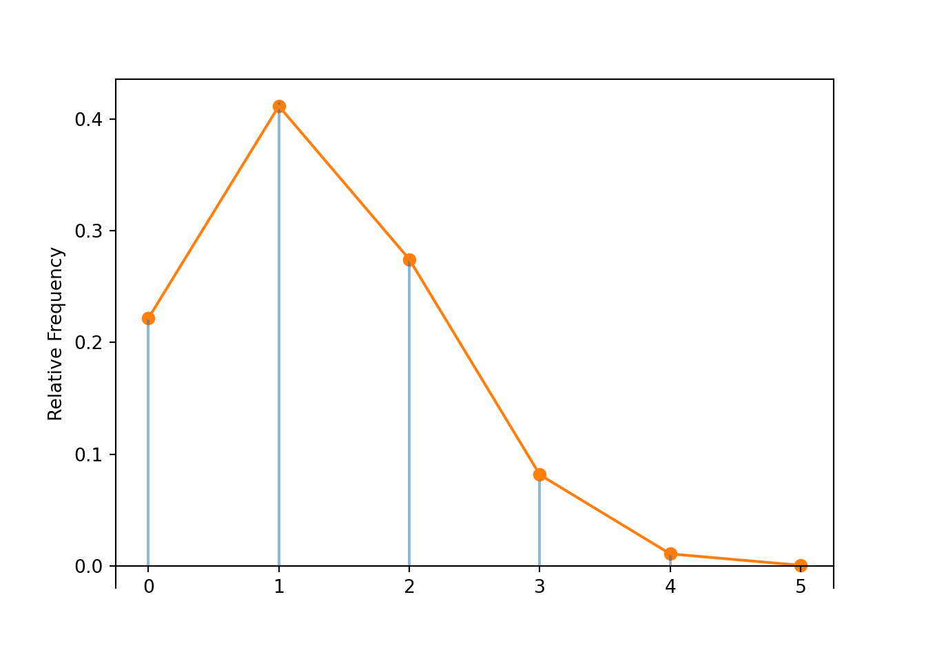
Compare to Table 4.1 and Figure 4.1. These represent the theoretical distribution of \(X\), but your simulation-based approximation should be similar (see our Symbulate output below).
For 10000 repetitions, the margin of error is roughly \(1/\sqrt{10000} = 0.01\) (or 0.02 following the recommendation in Section 3.6.2). Simulation results vary, but for most simulations adding and subtracting 0.01 to the simulated relative frequency of 0 will result in an interval that contains 0.237.
In this scenario, 23.7% of possible samples of 5 butterflies contain 0 tagged butterflies.
We could interpret the distribution is terms of relative frequencies as in the previous example: 39.6% of possible samples contain exactly 1 tagged butterfly, only about 1.6% of possible samples contain at least 4 tagged butterflies, etc. We can also interpret the distribution in terms of relative degrees of likelihood. The possible values, in order from most to least likely, are 1, 2, 0, 3, 4, 5.
The most likely value is 1, which is about 1.5 times more likely than 2.
2 is a little more likely (about 1.1 times) than 0.
0 is about 2.7 times more likely than 3
3 is about 6 times more likely than 4
4 is about 15 times more likely than 5
The following Symbulate code implements the simulation in Example 4.1. We define a box model with 13 tickets labeled 1 (“tagged”) and 39 labeled 0 (“not tagged”), and select 5 with replacement.
P = BoxModel({1: 13, 0: 39}, size =5, replace =True)P.sim(10)
Index
Result
0
(0, 1, 1, 0, 0)
1
(0, 1, 1, 1, 1)
2
(0, 0, 0, 1, 0)
3
(0, 1, 0, 0, 1)
4
(0, 1, 0, 0, 0)
5
(0, 0, 0, 1, 0)
6
(0, 0, 0, 1, 0)
7
(0, 1, 0, 1, 0)
8
(0, 0, 0, 0, 1)
...
...
9
(0, 0, 1, 0, 0)
Since the tickets are labeled 1/0 we can count the number of 1s (“tagged”) in a sample by summing.
X = RV(P, sum)(RV(P) & X).sim(10)
Index
Result
0
((0, 1, 0, 0, 0), 1)
1
((0, 0, 0, 1, 0), 1)
2
((0, 1, 1, 0, 1), 3)
3
((0, 0, 0, 0, 1), 1)
4
((1, 1, 0, 0, 1), 3)
5
((0, 0, 0, 1, 0), 1)
6
((0, 0, 0, 0, 1), 1)
7
((0, 1, 1, 0, 0), 2)
8
((0, 0, 0, 1, 0), 1)
...
...
9
((0, 1, 0, 0, 0), 1)
Now we simulate many values of \(X\).
x = X.sim(10000)x
Index
Result
0
0
1
1
2
2
3
1
4
0
5
1
6
2
7
1
8
3
...
...
9999
1
Approximate \(\textrm{P}(X = 0)\) with the relative frequency of 0; compare to the theoretical value 0.237.
x.count_eq(0) / x.count()
0.2436
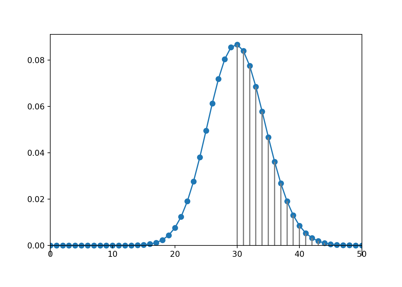
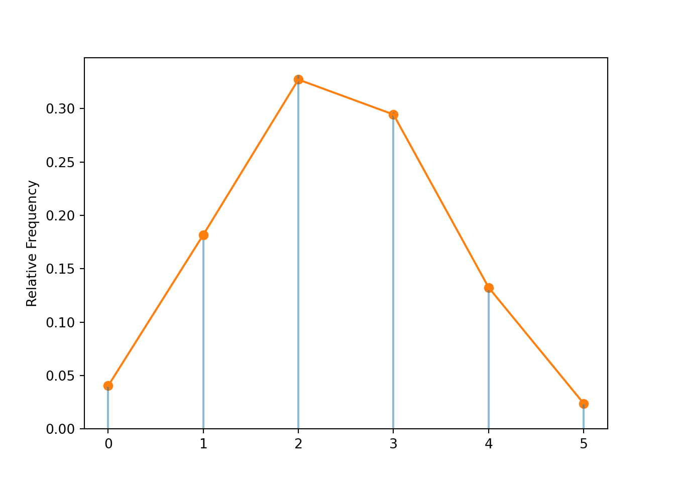
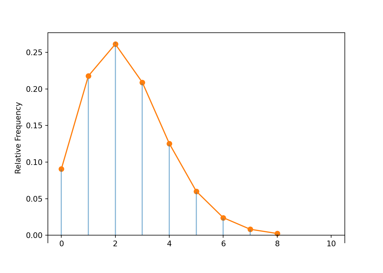
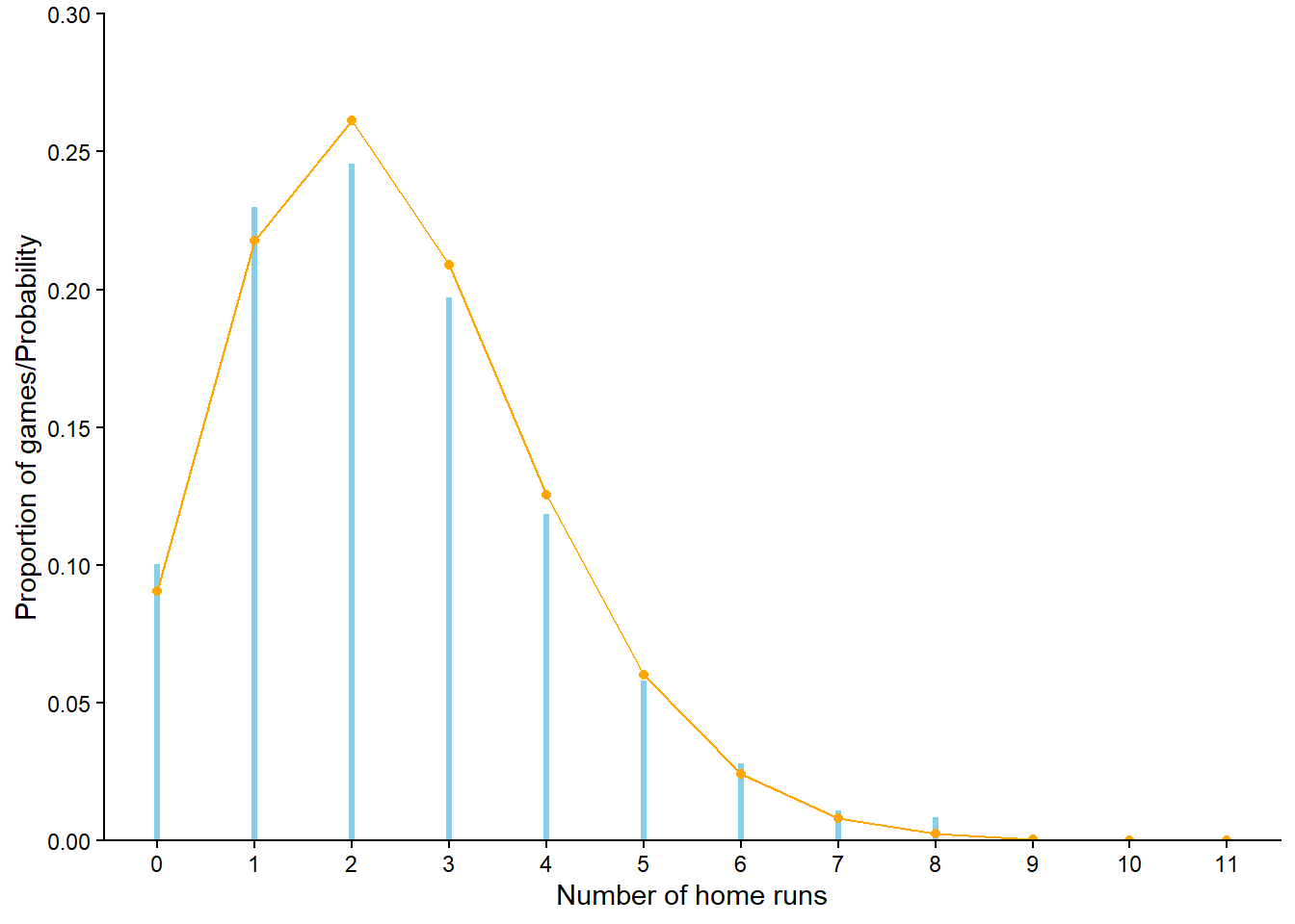
We can display the approximate distribution of \(X\) in a table or plot (x.plot()). Calling Binomial(5, 0.25).plot() overlays the theoretical distribution of \(X\), called the “Binomial(5, 0.25)” distribution (which we’ll discuss soon).
x.tabulate(normalize =True)
Value
Relative Frequency
0
0.2436
1
0.3968
2
0.2569
3
0.0878
4
0.0133
5
0.0016
Total
1.0
plt.figure();x.plot() # approximate distribution based on simulated valuesBinomial(5, 0.25).plot();# theoretical distribution
<symbulate.distributions.Binomial object at 0x00000191AA3CEE40>
plt.show()
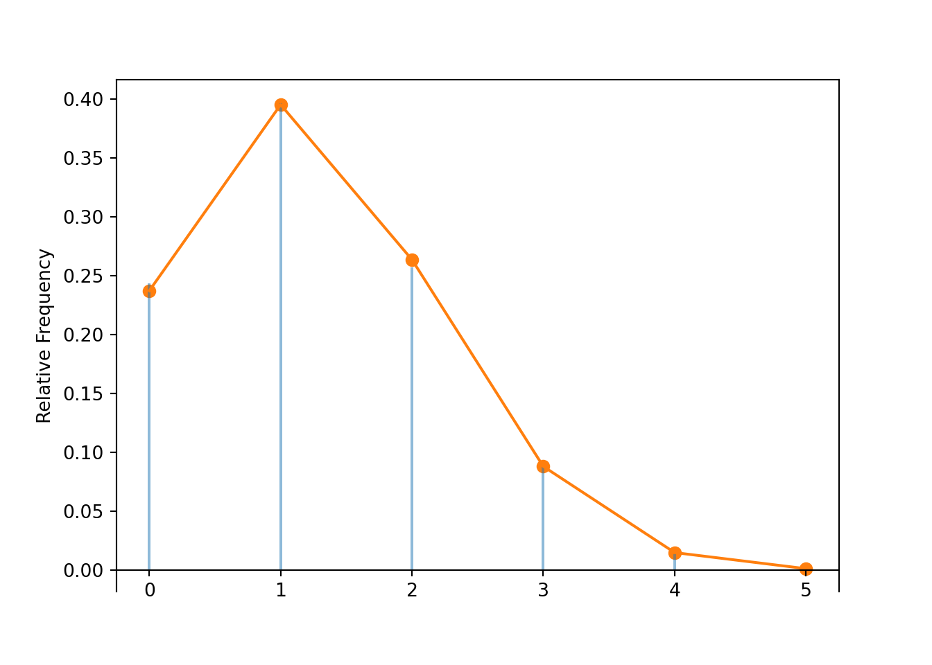
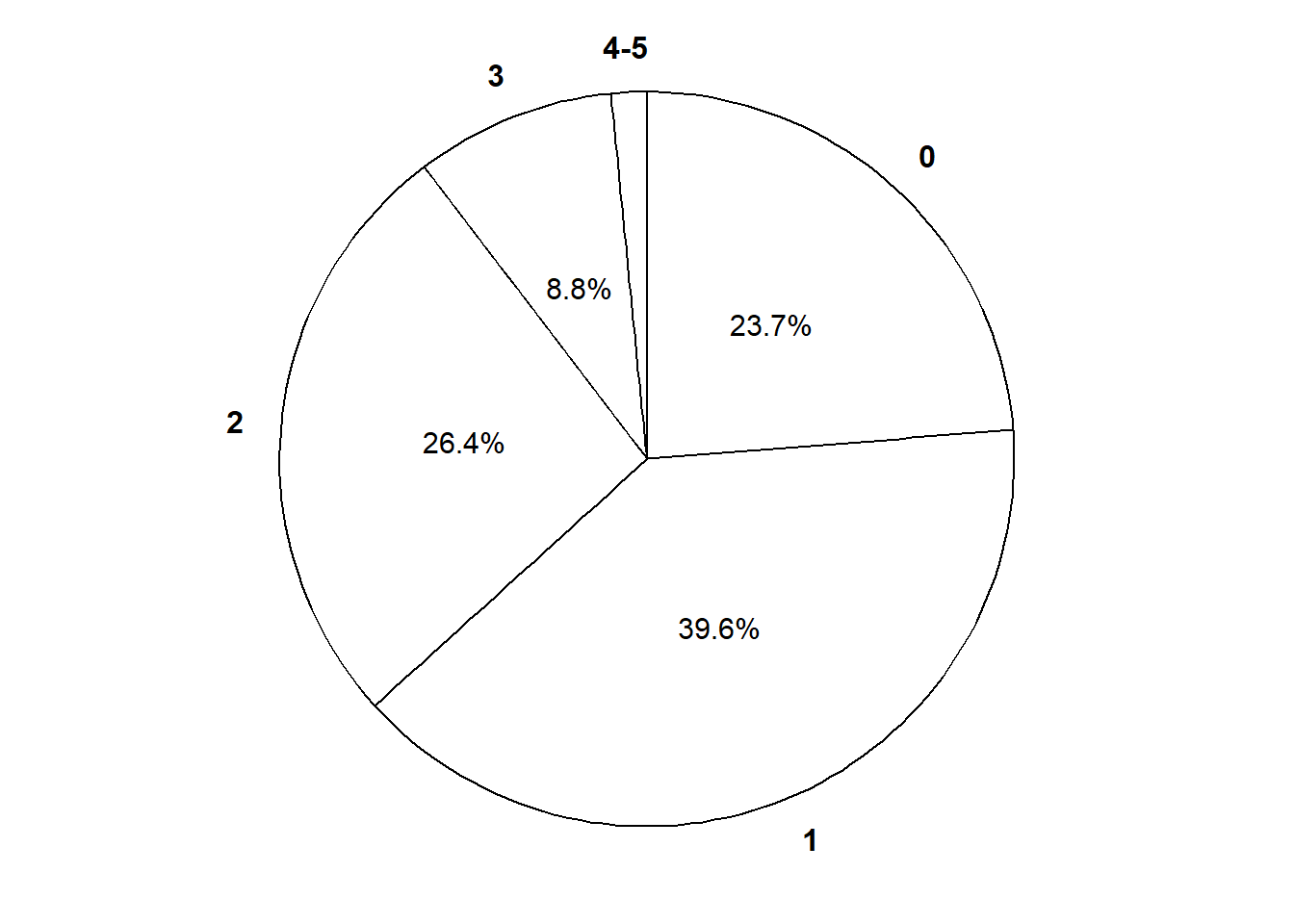
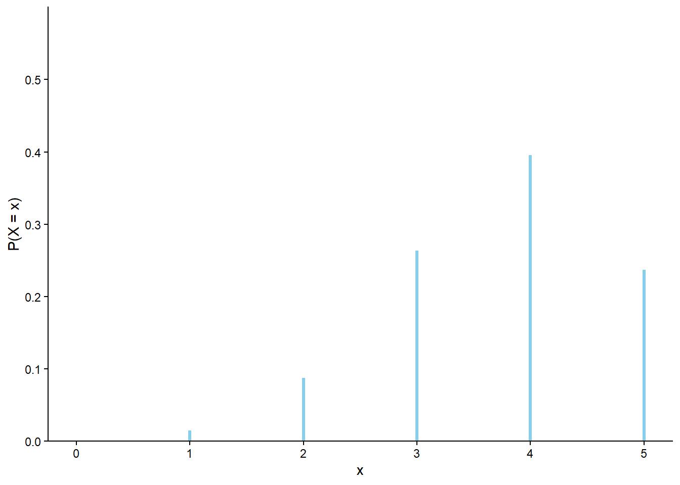
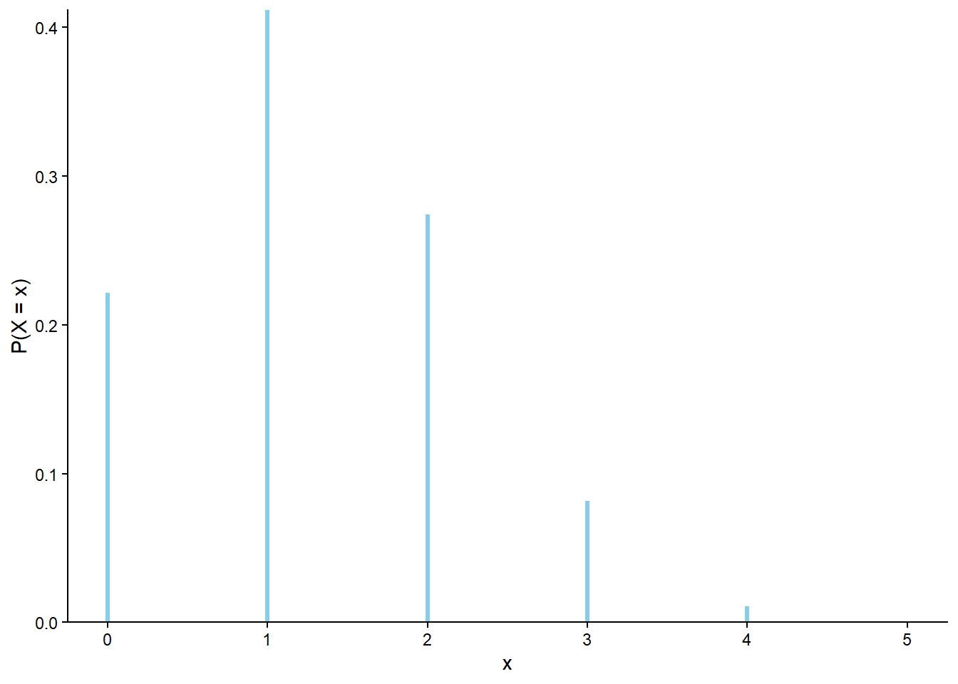
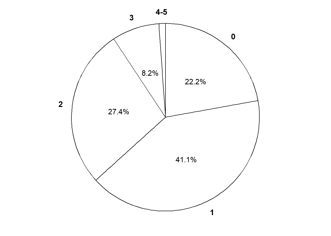
The marginal distribution of a discrete random variable \(X\) is often displayed in a table (like Table 4.1) or plot (like Figure 4.1 (a)) displaying the probability of the event \(\{X=x\}\) for each possible value \(x\). We can represent a marginal distribution of a discrete random variable with a spinner (like Figure 4.1 (b)) which returns possible values of the random variable with the appropriate probabilities.
Table 4.1: Table representing the the Binomial(5, 0.25) distribution, the theoretical distribution of \(X\) in Example 4.1.
x
P(X = x)
0
0.2373
1
0.3955
2
0.2637
3
0.0879
4
0.0146
5
0.0010
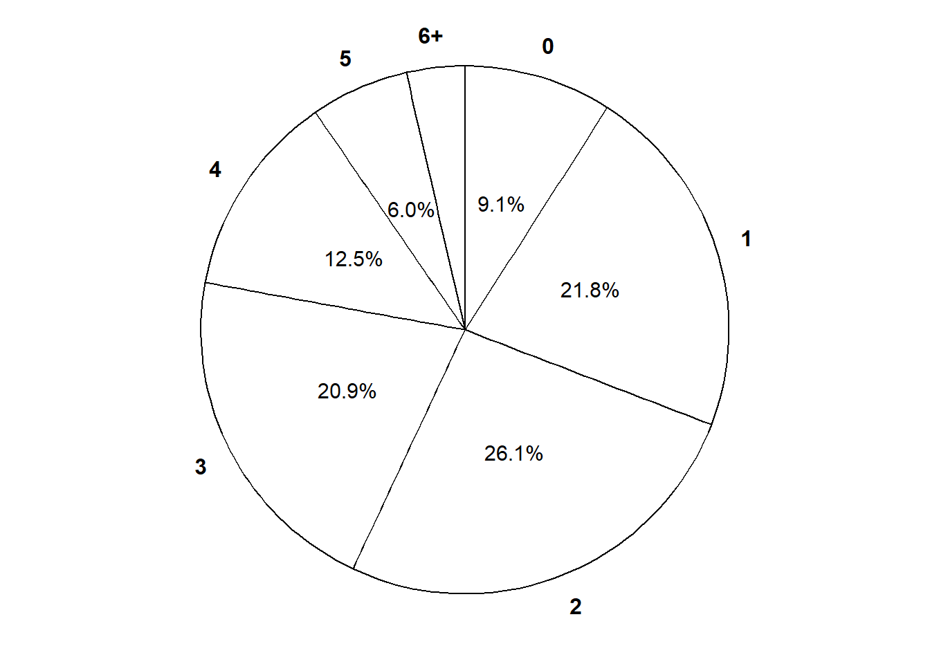
(a) Impulse plot
(b) Spinner; the values 4 and 5 have been grouped together and their total probability of 1.6% is not displayed.
Figure 4.1: Plot and spinner representing the the Binomial(5, 0.25) distribution, the theoretical distribution of \(X\) in Example 4.1.
4.2 Bernoulli trials and the Binomial situation
Some probabilistic situations are so common that the corresponding distributions have special names. Example 4.1 involves the “Binomial situation”, and the random variable \(X\) in Example 4.1 has a “Binomial distribution with parameters \(n = 5\) and \(p=0.25\)”.
We can describe the general Binomial situation in terms of a box model.
Imagine a box containing tickets where each ticket is labeled either 1 or 0.
Let \(p\) be the proportion of tickets in the box labeled 1.
Randomly select \(n\) tickets from the box with replacement.
Let \(X\) be the number of tickets in the sample that are labeled 1.
Since the tickets are labeled 1/0, the random variable \(X\) which counts the number of successes is equal to the sum of the 1/0 values on the tickets in the sample.
Then we say that \(X\) a Binomial distribution with parameters \(n\) and \(p\).
Binomial distributions are commonly used when sampling from a population.
Each individual in a population called be categorized as “success” (1) or not (0, “failure”).
“Success” is a generic term for whatever you’re interested in counting
“Success” is not necessarily good; for example if you’re counting the number of people who have died from a given cause then “success” equals death.
\(p\) is the population proportion of success
A random sample of size \(n\) is selected from the population (technically with replacement, but we will revisit later)
\(X\) is the number of successes in the sample
Then we say that \(X\) a Binomial distribution with parameters \(n\) and \(p\).
Example 4.2 Explain how Example 4.1 involves the Binomial situation, and identify the values of \(n\) and \(p\).
Solution (click to expand)
Solution 4.2.
There is a population of 52 butterflies and each butterfly is either tagged (success) or not (failure)
The proportion of tagged butterflies in the population is \(p=13/52 = 0.25\). Each time a butterfly is randomly selected, the marginal probability that the butterfly is tagged is \(p=0.25\).
A random sample of \(n=5\) butterflies is selected. Since the selections are made with replacement they are independent.
Every time a new butterfly is selected, with replacement the population proportion is 13/52=0.25 regardless of the results of the other selections.
In this case it is enough to just specify the population proportion \(0.25\) without knowing the population size
\(X\) counts the number of tagged butterflies in the sample, so \(X\) has a Binomial(5, 0.25) distribution.
Binomial situations can also be described in terms of “Bernoulli trials”.
Definition 4.1 In a sequence of Bernoulli(\(p\)) trials
There are only two possible outcomes, “success” (1) or not (0, “failure”), on each trial.
The unconditional/marginal probability of success is the same on every trial, and equal to \(p\).
The trials are independent.
Definition 4.2 Consider a fixed number, \(n\), of Bernoulli(\(p\)) trials and let \(X\) count the number of successes. The distribution of \(X\) is defined to be the Binomial(\(n, p\)) distribution.
A Binomial distribution is specified by two parameters:
\(n\) (an integer): the fixed number of Bernoulli trials, or the sample size
\(p\) (in \([0, 1]\)): the fixed marginal probability of success on each Bernoulli trial, or the population proportion of success
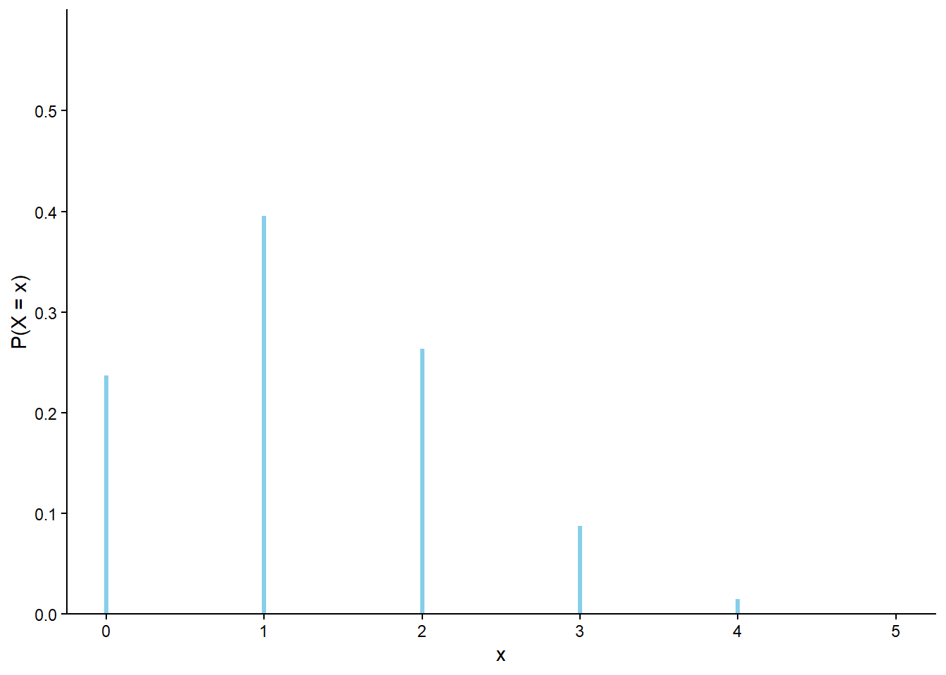
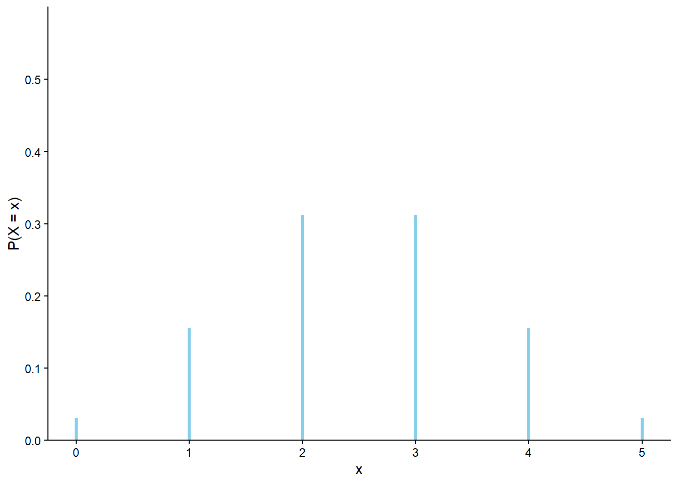
Example 4.3 Without doing any calculation or simulation, sketch a plot representing each of the following distributions, like Figure 4.1 (a) for the Binomial(5, 0.25) distribution. Explain your reasoning.
Binomial(5, 0.75)
Binomial(5, 0.5)
Binomial(5, 0.1)
The distribution of \(Y = 5-X\) for \(X\) in Example 4.1. Hint: what does \(Y\) represent in the butterfly context?
Solution (click to expand)
Solution 4.3.
The Binomial(5, 0.25) situation corresponds to a probability of success of 0.25 and of failure of 0.75, while the Binomial(5, 0.75) situation corresponds to a probability of success of 0.75 and of failure of 0.25. So going from Binomial(5, 0.25) to Binomial(5, 0.75) is just like switching the roles of success and failure. For example, seeing 0 successes in a Binomial(5, 0.25) situation is as likely as seeing 0 failures, and hence 5 successes, in a Binomial(5, 0.75) situation. To obtain a Binomial(5, 0.75) distribution, imagine “rotating” the Binomial(5, 0.25) distribution around \(n/2 = 2.5\); see Figure 4.2 (c).
In the Binomial(5, 0.5) situation, on each trial the probability of success is the same as failure, so we might expect the shape to be symmetric around \(n/2 = 2.5\), with the probabilities decreasing as \(x\) moves away from \(n/2\). See Figure 4.2 (b).
In the Binomial(5, 0.1) situation we only expect to see success in 1 in every 10 trials on average, so in only 5 trials we would most likely see 0 successes. So the probability is highest for \(x=0\) and then decreases as \(x\) increases. See Figure 4.2 (d)
The reasoning is similar to part 1. If \(X\) counts the number of tagged butterflies in the sample of 5, then \(Y=5-X\) counts the number of untagged butterflies. So \(Y\) also fits the Binomial situation, but untagged represents “success” (what \(Y\) counts) so the probability of success is 0.75. Therefore \(Y\) has a Binomial(5, 0.75) distribution as in part 1.
(a) \(p = 0.25\)
(b) \(p = 0.5\)
(c) \(p = 0.75\)
(d) \(p = 0.1\)
Figure 4.2: Binomial(\(n\), \(p\)) distributions with \(n=5\)
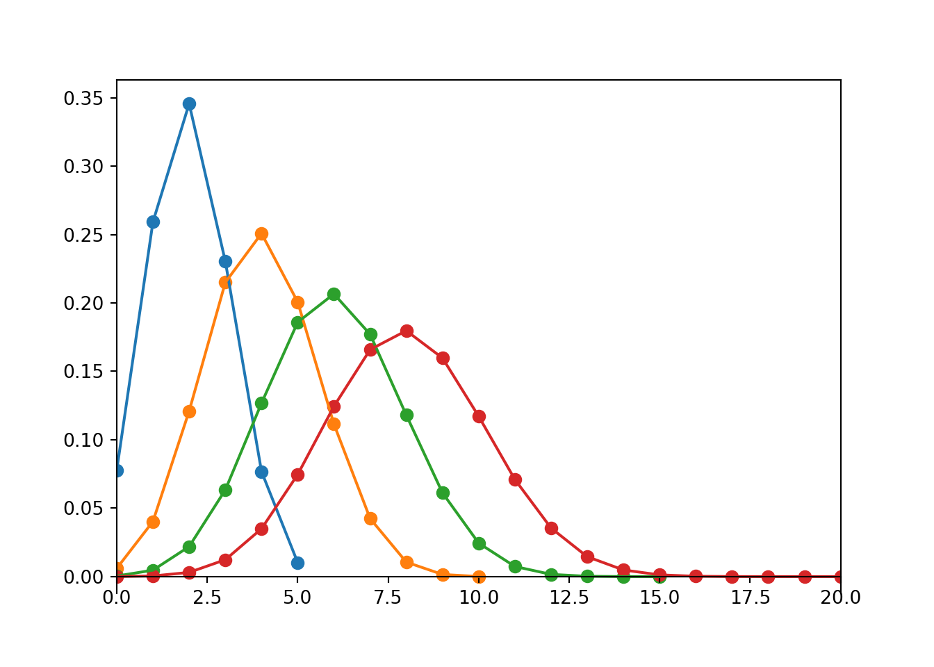
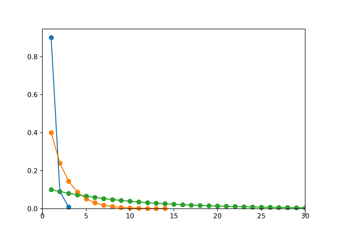
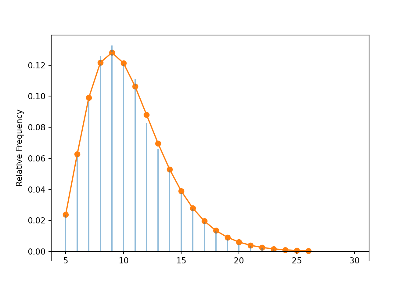
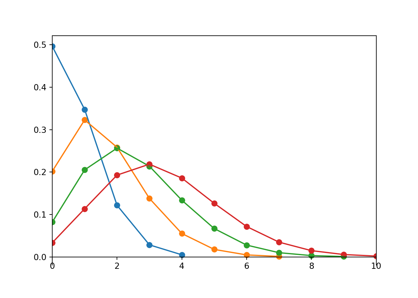
The exact shape of a Binomial distribution depends on \(n\) and \(p\). Figure 4.3 and Figure 4.4 display just a few examples of how changing \(n\) or \(p\) affects the shape of a Binomial distribution.
Figure 4.3: Binomial(\(n\), 0.4) distributions for (from left to right) \(n = 5, 10, 15, 20\).
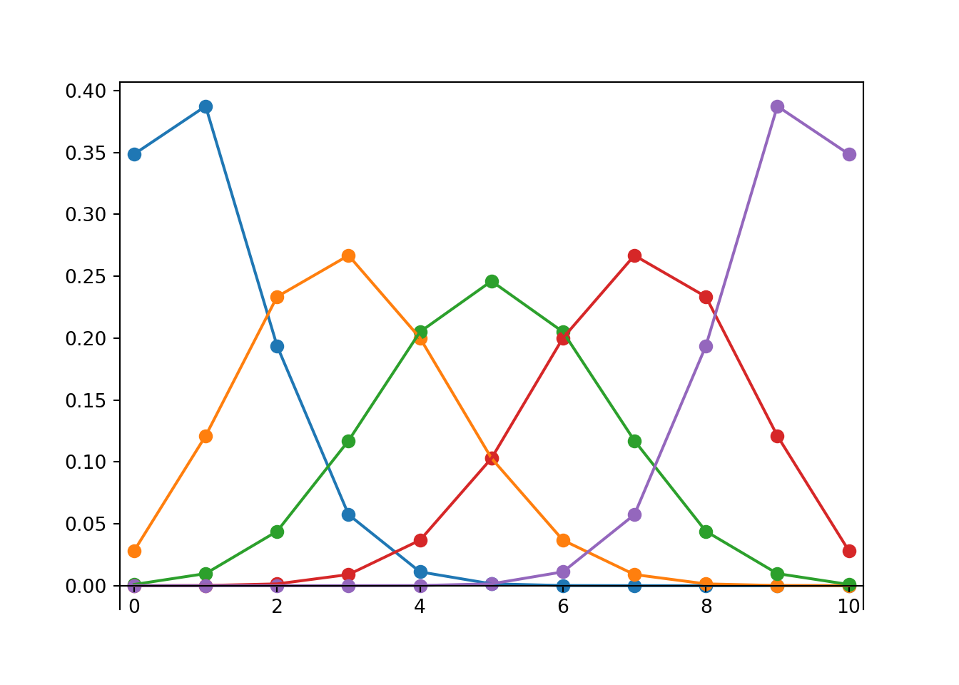
Figure 4.4: Binomial(10, \(p\)) distributions for (from left to right) \(p = 0.1, 0.3, 0.5, 0.7, 0.9\).
Example 4.4 In each of the following situations determine whether or not \(X\) has a Binomial distribution. If so, specify \(n\) and \(p\). If not, explain why not.
Roll a die 20 times; \(X\) is the number of times the die lands on an even number.
Roll a die 20 times; \(X\) is the number of times the die lands on 6.
Roll a die until it lands on 6; \(X\) is the total number of rolls.
Roll a die until it lands on 6 three times; \(X\) is the total number of rolls.
Roll a die 20 times; \(X\) is the sum of the numbers rolled.
Shuffle a standard deck of 52 cards (13 hearts, 39 other cards) and deal 5 without replacement; \(X\) is the number of hearts dealt. (Hint: be careful about why.)
Roll a fair six-sided die 10 times and a fair four-sided die 10 times; \(X\) is the number of 3s rolled (out of 20).
Solution (click to expand)
Solution 4.4.
Yes, Binomial(20, 0.5). Success = even.
Yes, Binomial(20, 1/6). Success = 6. The probability of success has to be the same on each trial. However, the probability of success does not have to be the same as the probability of failure.
Not Binomial; not a fixed number of trials. These are Bernoulli trials, but the random variable is not counting the number of successes in a fixed number of trials.
Not Binomial; not a fixed number of trials. These are Bernoulli trials, but the random variable is not counting the number of successes in a fixed number of trials.
Not Binomial; each trial has more outcomes than just success or failure, and the random variable is summing the values rather than counting successes.
Not Binomial, but be careful about the reason: the trials are not independent. The conditional probability that the second card is a heart given that the first card is a heart is 12/51, which is not equal to the conditional probability that the second card is a heart given that the first card is not a heart, 13/51. The trials are not independent. However, the unconditional probability of success is the same on each trial, \(p=13/52\). Recall Example 1.18 and the related discussion.
Not Binomial. Here the trials are independent, but the probability of success is not the same on each trial; it’s 1/6 for the six-sided die trials but 1/4 for the four sided-die trials. (We can write \(X = Y + Z\) where \(X\), the number of times the six-sided die lands on 3, has a Binomial(10, 1/6) distribution, and \(Y\), the number of times the four-sided die lands on 3, has a Binomial(10, 1/4) distribution and \(Y\) and \(Z\) are independent. But \(X\) itself does not have a Binomial distribution.)
Do not confuse the following two distinct assumptions of Bernoulli trials.
The probability of success is the same on each trial — this concerns the unconditional/marginal probability of each individual trial.
When sampling from a population, the probability of success will be the same on each trial regardless of whether the sampling is with or without replacement as long as all trials are sampled from the same population.
The trials are independent — this concerns joint or conditional probabilities for the collection of trials.
When sampling from a population, the trials will technically only be independent if the sampling is with replacement.
But when sampling without replacement, if the population size is much larger than the sample size then the trials will be nearly independent.
We will study Binomial distributions in much more detail as we go, including how to compute probabilities. For now, be sure to know how to identify the Binomial situation.
4.3 Probability mass functions
The marginal distribution of a discrete random variable \(X\) is often represented in a table or plot containing the probability of the event \(\{X=x\}\) for each possible value \(x\). In some cases the distribution has a “formulaic” shape and \(\textrm{P}(X=x)\) can be written explicitly as a function of \(x\).
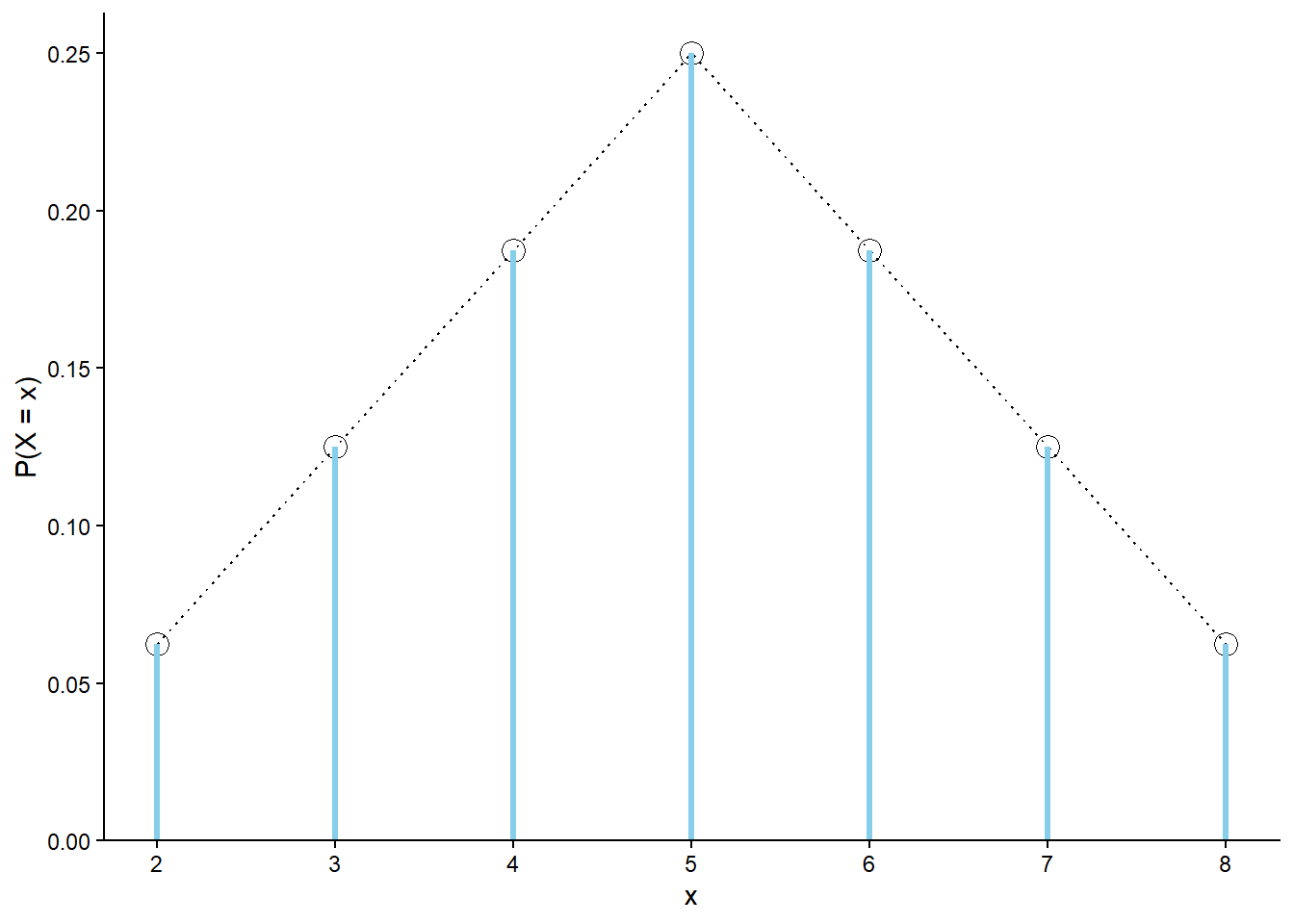
Recall Section 2.5 and consider again \(X\), the sum of two rolls of a fair four-sided die. See Figure 4.5; the probabilities of the possible values \(x\) follow a clear triangular pattern as a function of \(x\).
Warning
The dotted lines in Figure 4.5 emphasize the triangular pattern of \(\textrm{P}(X = X)\) as a function of \(x = 2, 3, 4, 5, 6, 7, 8\), but remember that \(\textrm{P}(X =x) = 0\) for other values of \(x\).
Figure 4.5: The marginal distribution of \(X\), the sum of two rolls of a fair four-sided die. The black dots represent the marginal probability mass function of \(X\).
For each possible value \(x\) of the random variable \(X\), \(\textrm{P}(X=x)\) can be obtained from the formula
That is, \(\textrm{P}(X = x) = p(x)\) for all \(x\). For example, \(\textrm{P}(X = 2) = 1/16 = p(2)\); \(\textrm{P}(X=5)=4/16=p(5)\); \(\textrm{P}(X=7.5)=0=p(7.5)\). To specify the distribution of \(X\) we could provide Table 2.7, or we could just provide the function \(p(x)\). Notice that part of the specification of \(p(x)\) involves the possible values of \(x\); \(p(x)\) is only nonzero for \(x=2,3, \ldots, 8\). Think of \(p(x)\) as a compact way of representing Table 2.7; given \(p(x)\) we could plug in the possible \(x\) values and construct Table 2.7. The function \(p(x)\) is called the probability mass function of the discrete random variable \(X\).
Definition 4.3 The probability mass2 function (pmf) of a discrete RV \(X\), defined on a probability space with probability measure \(\textrm{P}\), is a function \(p_X:\mathbb{R}\mapsto[0,1]\) which specifies each possible value of the RV and the probability that the RV takes that particular value: \(p_X(x)=\textrm{P}(X=x)\) for all \(x\).
The axioms of probability imply that a valid pmf must satisfy \[\begin{align*}
p_X(x) & \ge 0 \quad \text{for all $x$}\\
p_X(x) & >0 \quad \text{for at most countably many $x$ (the possible values, i.e., support)}\\
\sum_x p_X(x) & = 1
\end{align*}\]
The countable set of possible values of a discrete random variable \(X\), \(\{x: \textrm{P}(X=x)>0\}\), is called its support.
The pmf of a discrete random variable provides the probability of “equal to” events: \(\textrm{P}(X = x)\). Probabilities for other general events, e.g., \(\textrm{P}(X \le x)\) can be obtained by summing the pmf over the range of values of interest.
Example 4.5 Let \(Y\) be the larger of two rolls of a fair four-sided die. Find the probability mass function of \(Y\).
Solution (click to expand)
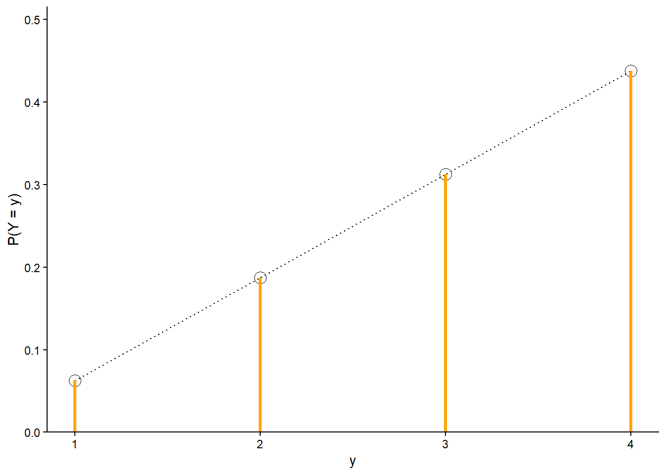
Solution 4.5. Recall Table 2.15 and Figure 2.17. As a function of \(y=1, 2, 3, 4\), \(\textrm{P}(Y=y)\) is linear with slope 2/16 passing through the point (1, 1/16); see Figure 4.6. The pmf of \(Y\) is
For any \(y\), \(\textrm{P}(Y=y) = p_Y(y)\). For example, \(\textrm{P}(Y=2) = 3/16 = p_Y(2)\) and \(\textrm{P}(Y = 3.3) = 0 = p_Y(3.3)\).
Figure 4.6: The marginal distribution of \(Y\), the larger (or common value if a tie) of two rolls of a fair four-sided die. The black dots represent the marginal probability mass function of \(Y\). The dotted lines emphasize the linear pattern, but the actual probability is 0 between possible values.
When there are multiple discrete random variables of interest, we usually identify their marginal pmfs with subscripts: \(p_X, p_Y, p_Z\), etc.
Example 4.6 Donny Dont provides two answers to Example Example 4.5. Are his answers correct? If not, why not?
\(p_Y(y) = \frac{2y-1}{16}\)
\(p_Y(x) = \frac{2x-1}{16},\; x = 1, 2, 3, 4\), and \(p_Y(x)= 0\) otherwise.
Solution (click to expand)
Solution 4.6.
Donny’s solution is incomplete; he forgot to specify the possible values. It’s possible that someone who sees Donny’s expression would think that \(p_Y(2.5)\) is equal to 4/16 instead of 0. You don’t necessarily always need to write “0 otherwise”, but do always clearly identify the possible values.
Donny’s answer is actually correct, though maybe a little confusing. The important place to put a \(Y\) is the subscript of \(p\): \(p_Y\) identifies this function as the pmf of the random variable \(Y\), the larger of the two rolls, as opposed to any other random variable that might be of interest. The argument of \(p_Y\) is just a dummy variable that defines the function. As an analogy, \(g(u)=u^2\) is the same function as \(g(x)=x^2\); it doesn’t matter which symbol defines the argument. It is convenient to represent the argument of the pmf of \(Y\) as \(y\), and the argument of the pmf of \(X\) as \(x\), but this is not necessary. Donny’s answer does provide a way of constructing Table 2.15 and Figure 4.6.
In some scenarios we can derive the pmf of a discrete random variable using probability rules.
Example 4.7 Maya is a basketball player who makes 40% of her three point field goal attempts. Suppose that she attempts three pointers until she makes one and then stops. Let \(X\) be the total number of shots she attempts. Assume shot attempts are independent.
Can Maya’s attempts be considered Bernoulli trials?
Explain why \(X\) does not have a Binomial distribution.
What are the possible values that \(X\) can take? Is \(X\) discrete or continuous?
Compute and interpret \(\textrm{P}(X=1)\).
Compute and interpret \(\textrm{P}(X=2)\).
Compute and interpret \(\textrm{P}(X=3)\).
Compute and interpret \(\textrm{P}(X=4)\).
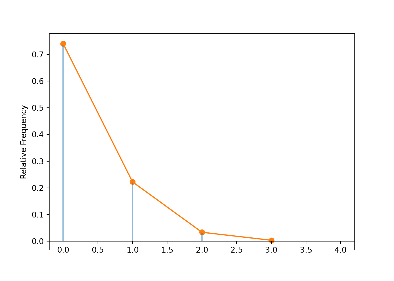
Find the probability mass function of \(X\).
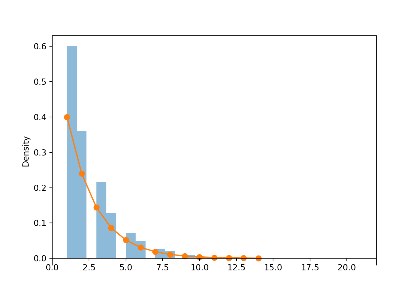
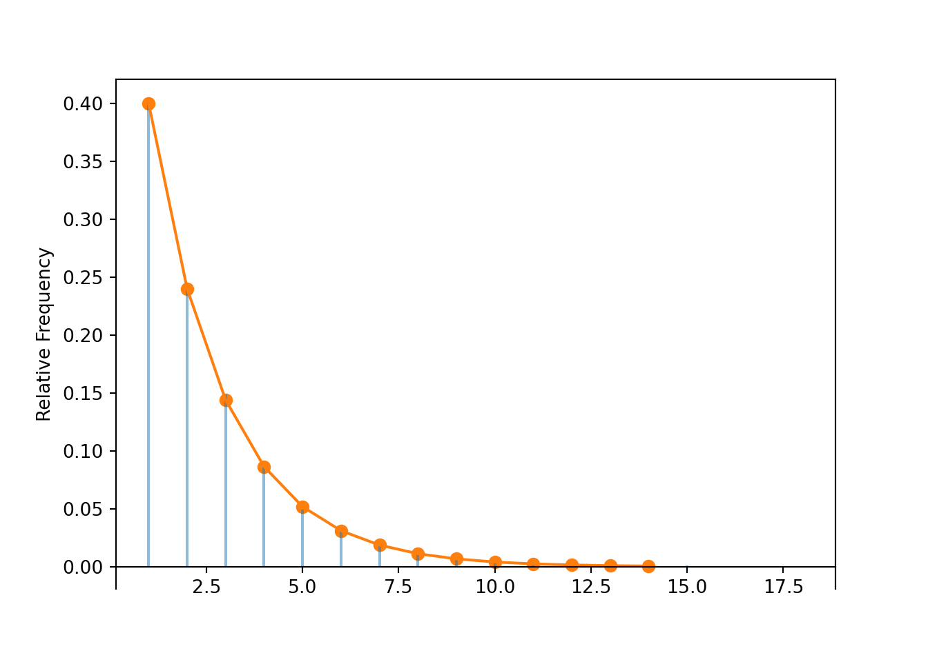
Construct a table, plot, and spinner representing the distribution of \(X\).
Compute \(\textrm{P}(X>5)\). Can you think of a way to do this without summing several terms?
Solution (click to expand)
Solution 4.7.
Yes, these are Bernoulli trials: each attempt results in success or failure, the probability of success on any attempt is 0.4, and the attempts are assumed to be independent.
There are Bernoulli trials but \(X\) does not have a Binomial distribution since the number of trials is not fixed.
\(X\) can take values 1, 2, 3, \(\ldots\). Even though it is unlikely that \(X\) is very large, there is no fixed upper bound. Even though \(X\) can take infinitely many values, \(X\) is a discrete random variable because it takes countably many possible values.
In order for \(X\) to be 1, Maya must make her first attempt, so \(\textrm{P}(X = 1) = 0.4\). If Maya does this every practice, then in about 40% of practices she will make a three pointer on her first attempt.
In order for \(X\) to be 2, Maya must miss her first attempt and make her second. Since the attempts are independent \(\textrm{P}(X=2)=(1-0.4)(0.4)=0.24\). If Maya does this every practice, then in about 24% of practices she will make her first three pointer on her second attempt.
In order for \(X\) to be 3, Maya must miss her first two attempts and make her third. Since the attempts are independent \(\textrm{P}(X=3)=(1-0.4)(1-0.4)(0.4)=(1-0.4)^2(0.4)=0.144\). If Maya does this every practice, then in about 14.4% of practices she will make her first three pointer on her third attempt.
In order for \(X\) to be 4, Maya must miss her first three attempts and make her fourth. Since the attempts are independent \(\textrm{P}(X=4)=(1-0.4)(1-0.4)(1-0.4)(0.4)=(1-0.4)^3(0.4)=0.0864\). If Maya does this every practice, then in about 8.6% of practices she will make her first three pointer on her fourth attempt.
The previous parts suggest a general pattern. In order for \(X\) to take value \(x\), the first success must occur on attempt \(x\), so the first \(x-1\) attempts must be failures. Therefore, \(\textrm{P}(X=x)\) as a function of \(x\) is given by the pmf \[
p_X(x) = (1-0.4)^{x-1}(0.4), \qquad x = 1, 2, 3, \ldots
\]
We could compute \(\textrm{P}(X > 5)\) as \(1 - \textrm{P}(X \le 5) = 1 - (\textrm{P}(X = 1) + \cdots +\textrm{P}(X = 5))\). A quicker way is to realize that given the setup Maya requires more than 5 attempts to obtain her first success (that is, \(X > 5\)) if and only if the first 5 attempts are failures. Therefore, \[
P(X > 5) = \textrm{P}(\text{first 5 attempts are failures}) = (1-0.4)^5 = 0.078
\]
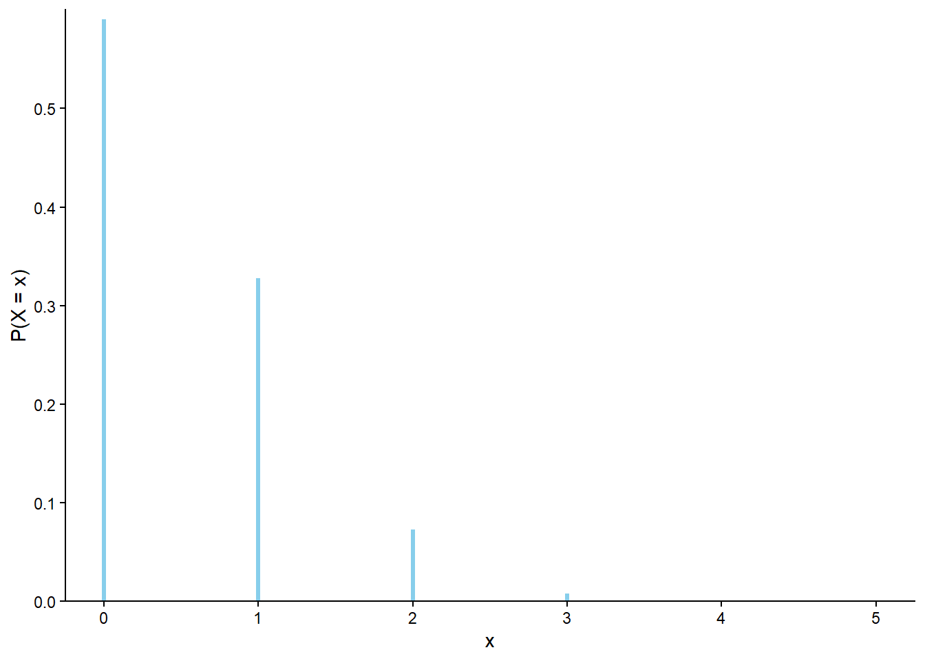
Table 4.2: Table representing the the Geometric(0.4) distribution, the theoretical distribution of \(X\) in Example 4.7.
x
P(X = x)
1
0.4000
2
0.2400
3
0.1440
4
0.0864
5
0.0518
6
0.0311
7
0.0187
8
0.0112
9
0.0067
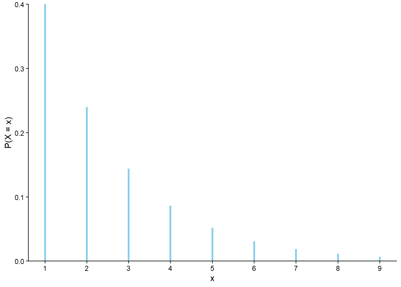
(a) Impulse plot
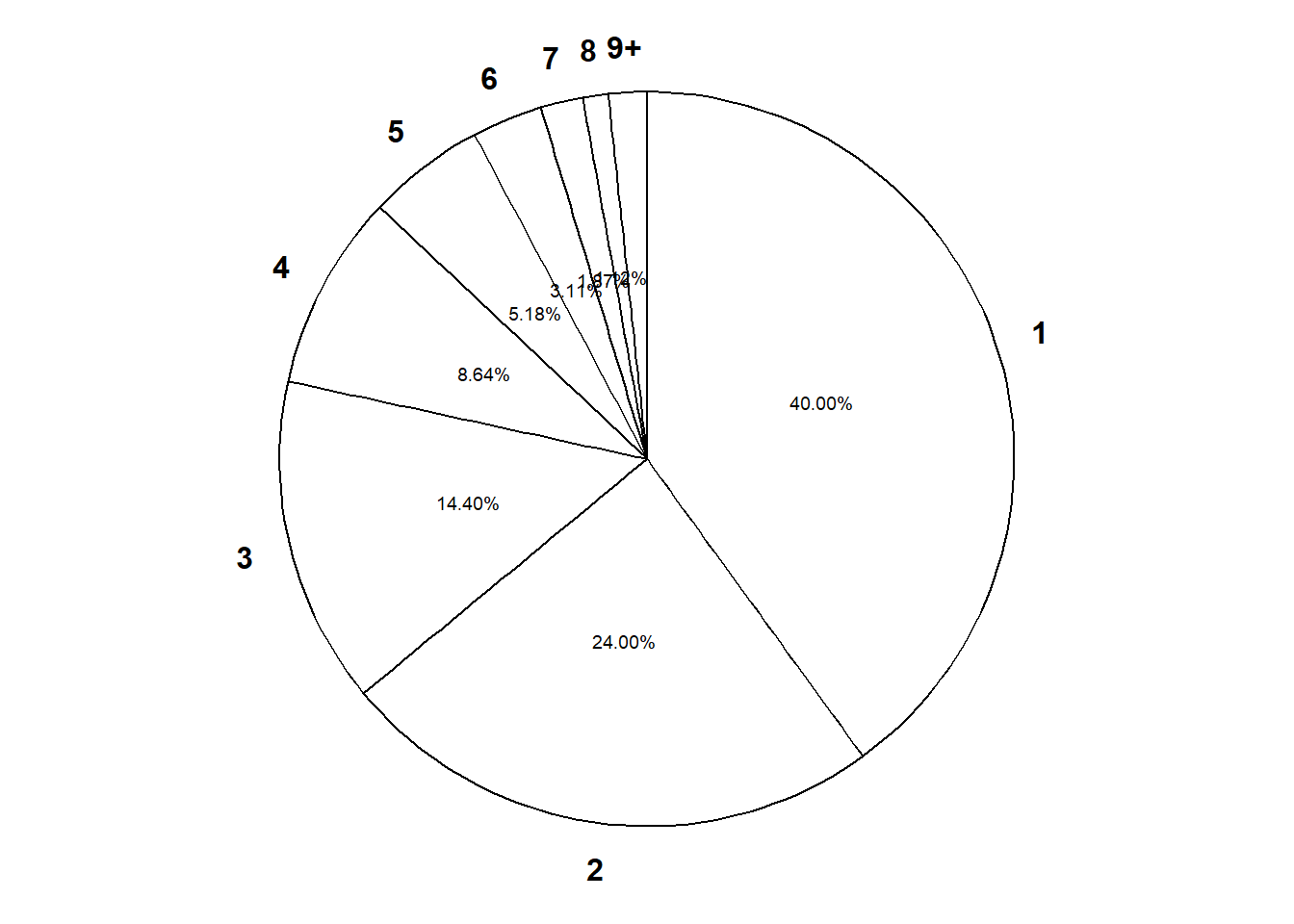
(b) Spinner; the values 9+ have been grouped together
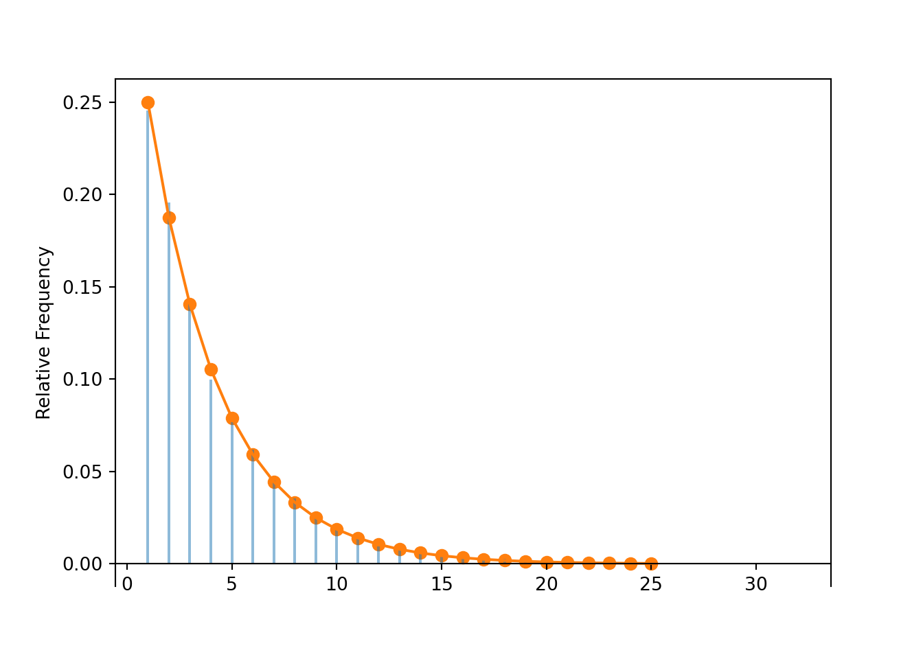
Figure 4.7: Plot and spinner representing the the Geometric(0.4) distribution, the theoretical distribution of \(X\) in Example 4.7.
The following Symbulate code conducts a simulation for Example 4.7. The value of \(X\) depends on a sequence of Bernoulli trials, but the number of trials is not know in advance. We can simulate Bernoulli trials of unspecified length in Symbulate using Bernoulli(p) ** inf; each trial results in either 1 (success) or 0 (failure). (The inf implies “infinite”, but in reality Symbulate will keep simulating as many Bernoulli trials as needed.) Given a sequence of Bernoulli trials (of any length) we define a function count_until_first_success that outputs the number of trials until the first success and then use it to define a RVX.
def count_until_first_success(omega):for i, w inenumerate(omega):if w ==1:return i +1# the +1 is for zero-based indexingP = Bernoulli(0.4) ** infX = RV(P, count_until_first_success)
Now we simulate many values of \(X\) and summarize the results; the simulation results are consistent with the theoretical distribution represented by Table 4.2 and Figure 4.7.
x = X.sim(10000)x.tabulate(normalize =True)
Value
Relative Frequency
1
0.4
2
0.24
3
0.144
4
0.0857
5
0.048
6
0.0328
7
0.0186
8
0.0145
9
0.0066
10
0.0043
11
0.0025
12
0.0014
13
0.0005
14
0.0006
15
0.0001
16
0.0001
17
0.0001
20
0.0001
21
0.0001
...
...
21
0.0001
Total
1.0
x.plot()Geometric(0.4).plot() # Overlay the theoretic pmf
<symbulate.distributions.Geometric object at 0x00000191AA2BBB60>
plt.show()
Many commonly encountered probability mass functions correspond to named distributions. The distribution of \(X\) in Example 4.7 is called the “Geometric(0.4)” distribution. We’ll discuss Geometric distributions in more detail soon.
The probability mass functions of many commonly encountered named distributions are built in to Symbulate and can be called as Distribution(parameters).pmf(x). For example, we can use Symbulate to compute \(\textrm{P}(X = 3) = 0.144\) in Example 4.7.
Geometric(0.4).pmf(3)
np.float64(0.144)
4.4 Simulating from a marginal distribution
Recall from Section 3.14 that there are two basic methods for simulating a value \(x\) of a random variable \(X\).
Simulate from the probability space. Simulate an outcome \(\omega\) from the underlying probability space and set \(x = X(\omega)\).
Simulate from the distribution. Simulate a value \(x\) directly from the distribution of \(X\).
Example 4.8 Recall Example 4.1 and the discussion and Symbulate code following it.
Which method did we use to simulate values of \(X\)?
Describe how could we simulate values of \(X\) using the other method.
Write the Symbulate code to simulate values of \(X\) using the other method and summarize the simulated values. Is the simulation consistent with our early simulation?
Solution (click to expand)
Solution 4.9.
We used the “simulate from the probability space method”. We simulated a sequence of five success/failure trials (outcome \(\omega\)) and counted the number of successes (\(X(\omega)\)).
The spinner in Figure 4.1 (b) represents the distribution of \(X\). To simulate a value of \(X\) from the distribution, we just spin this spinner once.
See the Symbulate code below. We can “simulate from the distribution” in Symbulate by defining X = RV(Binomial(5, 0.25)); read this as “\(X\) is a random variable with a Binomial(5, 0.25) distribution”. This code basically says that values of \(X\) will be simulated using the spinner in Figure 4.1 (b).
X = RV(Binomial(5, 0.25))X.sim(10)
Index
Result
0
0
1
2
2
1
3
1
4
1
5
1
6
0
7
2
8
2
...
...
9
2
X.sim(10000).tabulate(normalize =True)
Value
Relative Frequency
0
0.2405
1
0.3919
2
0.2638
3
0.0892
4
0.014
5
0.0006
Total
1.0
The “simulate from the distribution” method corresponds to constructing a spinner representing the marginal distribution of \(X\) and spinning it once to generate \(x\). This method does require that the distribution of \(X\) is known. However, as we will see in many examples, it is common to specify the distribution of a random variable directly without defining the underlying probability space.
Many commonly encountered distributions have special names, and in Symbulate we can define a random variable to have a specific named distribution through code of the form RV(Distribution(parameters)). For an unnamed discrete distribution, specified as a table of possible values and probabilities, BoxModel with the probs option can be used (when there are finitely many possible values).
Example 4.9 Recall Example 4.7. Maya is a basketball player who makes 40% of her three point field goal attempts. Suppose that she attempts three pointers until she makes one and then stops. Let \(X\) be the total number of shots she attempts. Assume shot attempts are independent.
Specify how you could simulate a value of \(X\) using the “simulate from the probability space” method.
Specify how you could simulate a value of \(X\) using the “simulate from the distribution” method.
Explain how you could use simulation to approximate the distribution of \(X\).
Write Symbulate code to approximate the distribution of \(X\) using the “simulate from the distribution” method.
Solution (click to expand)
Solution 4.9.
Spin a spinner that lands on success with probability 0.4 (and failure otherwise) until it lands on success then stop; \(X\) is the number of spins. This is the method represented by the Symbulate code after Example 4.7.
Construct a spinner representing the probability mass function in part 7 (see Figure 4.7) then spin it once; the resulting value is \(X\).
Simulate many values of \(X\) (using either method) then summarize the simulated values: For each possible value, compute the simulated relative frequency, e.g. to approximate \(\textrm{P}(X = 3)\) count the number of repetitions resulting in an \(X\) value of 3 and divide by the total number of repetitions.
See below. The simulation results are consistent with the Example 4.7 and the simulation based on the “simulate from the probability space” method.
X = RV(Geometric(0.4))x = X.sim(10000)x
Index
Result
0
3
1
2
2
4
3
9
4
2
5
3
6
1
7
5
8
4
...
...
9999
3
x.tabulate(normalize =True)
Value
Relative Frequency
1
0.4008
2
0.2402
3
0.1489
4
0.0863
5
0.0493
6
0.0301
7
0.0187
8
0.0108
9
0.0063
10
0.0032
11
0.0019
12
0.0011
13
0.0006
14
0.0005
15
0.0008
16
0.0004
18
0.0001
Total
1.0
x.plot()Geometric(0.4).plot() # Overlay the theoretic pmf
<symbulate.distributions.Geometric object at 0x00000191AA37CE90>
plt.show()
4.5 Binomial Distributions
A Binomial(\(n\), \(p\)) distribution has a probability mass function that depends on \(n\) and \(p\) whose form—which we will see later3—is determined by the assumptions of Definition 4.2. The following code shows how we can use Symbulate to compute probabilities involving a random variable \(X\) with a Binomial(5, 0.25) distribution as in Example 4.1.
Binomial(n =5, p =0.25).pmf(0)
np.float64(0.2373046874999998)
We can plug in all possible values of \(X\) to compute the Binomial(5, 0.25) pmf.
The following code achieves the same purpose, but uses list comprehension and displays the results in a table.
xs =list(range(5+1))pmf_x = [Binomial(n =5, p =0.25).pmf(x) for x in xs]print(tabulate({'x': xs,'Binomial(5, 0.25) pmf(x)': pmf_x}, headers ='keys', floatfmt=".3f"))
If we know a random variable has a Binomial distribution, then we can use Symbulate as a probability calculator. Therefore, the key is to identify the Binomial situation and the relevant parameters.
Example 4.10 Use Symbulate to compute the following probabilities, then interpret the values in context.
Shuffle a standard deck of 52 cards and deal 5 with replacement. What is the probability that there are no hearts among the cards dealt?
Shishito peppers are typically relatively mild, but about 10% are spicy. If these peppers are sold in packs of 20, what is the probability that a pack contains at least one spicy pepper?
About 70% of major league baseball pitchers are right-handed. If 13 pitchers are selected at random, what is the probability that at most 8 are right-handed?
Solution (click to expand)
Solution 4.10.
The context is different, but probabilistically this situation is the same as Example 4.1. If \(X\) is the number of hearts among the 5 cards dealt, then \(X\) has a Binomial(5, 0.25) distribution, and \(\textrm{P}(X=0) = 0.237\). About 23.7% of five-card-hands, dealt with replacement, will contain no hearts.
If \(X\) is the number of spicy peppers in a twenty-pepper-pack then \(X\) has a Binomial(20, 0.1) distribution. We want \(\textrm{P}(X\ge 1)\) which we can compute, using the complement rule, as \(1 - \textrm{P}(X = 0)\): either at least one pepper in the pack is spicy or none of them are. In Symbulate, 1 - Binomial(20, 0.1).pmf(0) yields 0.878. About 88% of 20-pepper-packs of Shishito peppers contain at least one spicy pepper. In other words, a pack is about 7 times more likely than not to contain at least one spicy pepper.
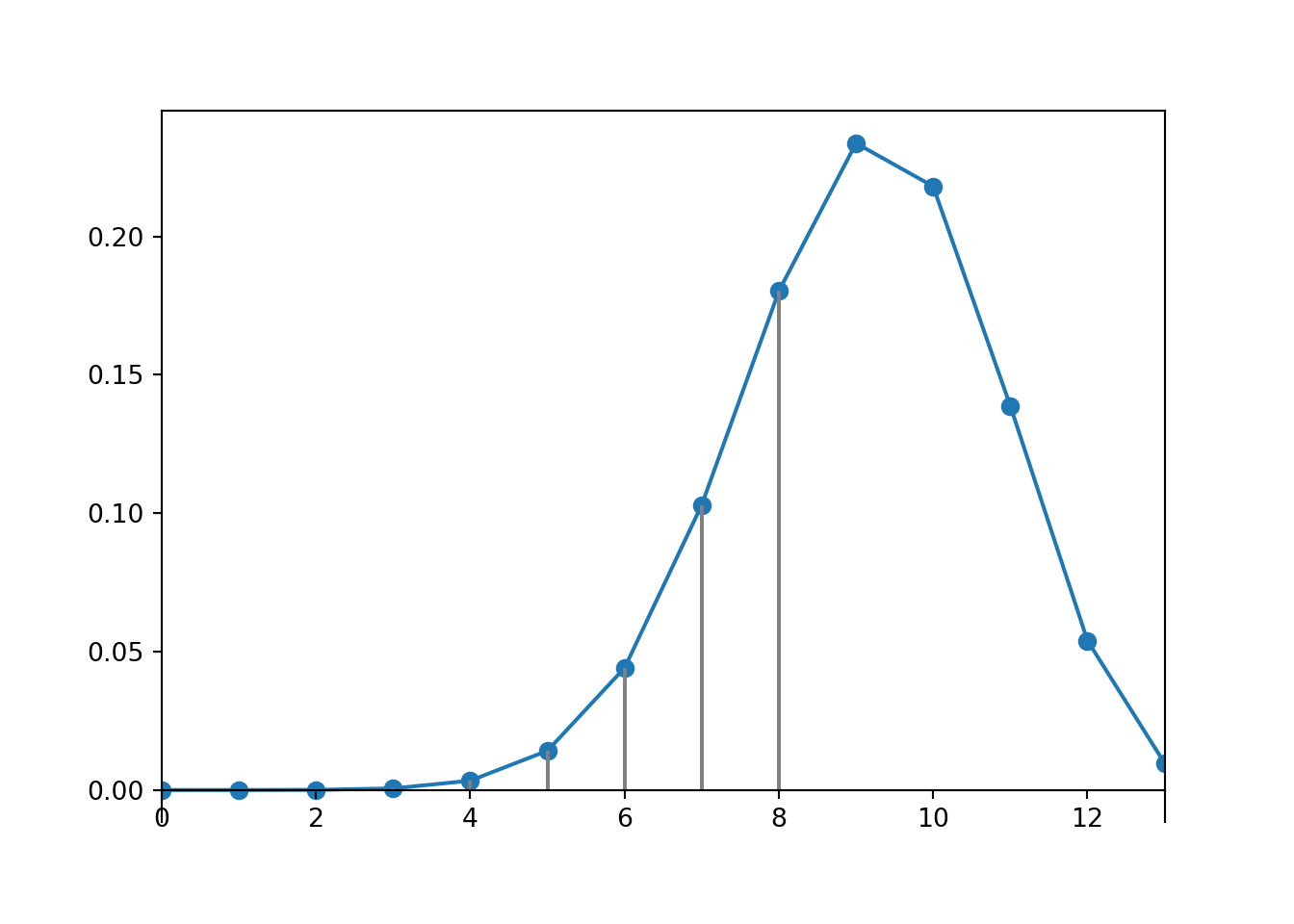
If \(X\) is the number of the 13 pitchers that are right-handed, then \(X\) has a Binomial(13, 0.70) distribution. We want \(\textrm{P}(X \le 8)\), which we can compute as \(\textrm{P}(X = 0) + \textrm{P}(X = 1) + \cdots \textrm{P}(X = 8)\). Symbulate code (see below) yields 0.346. About 35% of groups of 13 pitchers will have at most 8 right-handed pitchers.
The pmf directly provides probabilities of “equal to” events, but we can obtain probabilities of other events by summing appropriately, as in the following Symbulate code.
The probability mass function (pmf) returns “equal to” probabilities: \(\textrm{P}(X = x)\). The cumulative distribution function (cdf) provides “less than or equal to” probabilities \(\textrm{P}(X \le x)\). We can use the cdf method in Symbulate to shortcut summing. (We will discuss cumulative distribution functions in much more detail for continuous random variables.)
Binomial(13, 0.7).cdf(8)
np.float64(0.3456864392985002)
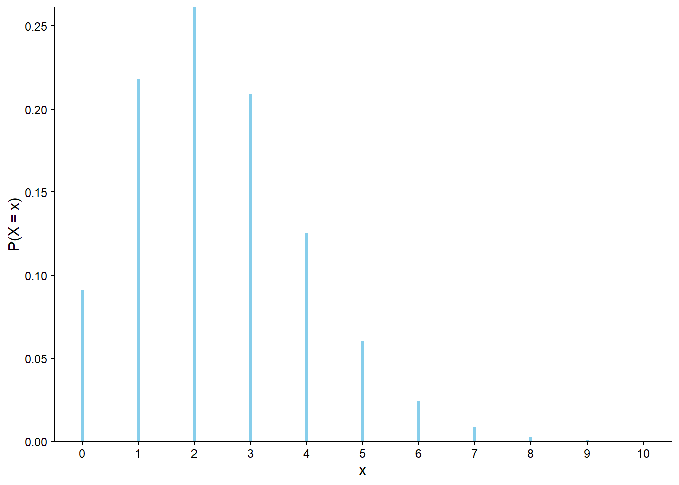
Figure 4.8 displays the Binomial(13, 0.7) pmf with \(p(x)\) for \(x\le 8\) highlighted. Binomial(13, 0.7).cdf(8) computes the sum of the probabilities represented by the spikes for \(x\le 8\).
Binomial(13, 0.7).plot().shade(le =8)
<symbulate.distributions.Binomial object at 0x00000191AACEF040>
Figure 4.8: Binomial(13, 0.7) pmf, with \(p(x)\) for \(x \leq 8\) highlighted
Note that cdf(x) by definition returns \(\textrm{P}(X \le x)\). We can obtain other probabilities by using the complement rule or subtracting. For example, 1-Binomial(13, 0.7).cdf(8) returns \(1 - \textrm{P}(X\le 8)=\textrm{P}(X > 8) = \textrm{P}(X \ge 9)\).
Example 4.11 Roy, a baseball player, tells his coach: “Throughout my career my probability of getting a hit in an at bat has been 0.250. But ever since baseball season ended, I’ve been practicing really hard and I have definitely improved my hitting”. The coach needs some convincing and decides to let Roy have 100 at bats to convince him. Let \(X\) be the number of hits Roy gets in the 100 at bats.
You can assume Roy’s probability of getting a hit on any single at bat, \(p\) is the same for each at bat and that the at bats are independent (and you can ignore baseball context like walks/etc. and assume that there is no funny business in data collection).
What is the distribution of \(X\)? What is the distribution of \(X\)if Roy has not improved?
Suppose the coach decides that if Roy gets at least 30 hits he’ll be convinced. What is the probability that Roy convinces the coach that he has improved even if he has not really improved?
Suppose that Roy really has improved and his probability of getting a hit in an at bat is 0.300. What is the probability that Roy convinces the coach that he has improved?
Suppose the coach wants the probability in part 2 to be 0.01. What should his threshold for convincing—which was 30 in the part 2—be? Should the threshold be greater or less than 30?
Use Symbulate and trial and error to find a threshold which gets the probability in part 2 as close to 0.01 without going over.
The coach decides to use the threshold from the previous part. Suppose that Roy really has improved and his probability of getting a hit in an at bat is 0.300. What is the probability that Roy convinces the coach that he has improved? How does this compare to part 3?
Repeat parts 4 and 5 assuming Roy has 400 at bats. How do the values change?
Now Roy actually takes 100 at bats and gets hits in 38 at bats. What is the probability that Roy would get at least 38 hits if he really hadn’t improved? Did he necessarily improve? Are you convinced that he improved? Explain.
Solution (click to expand)
Solution 4.11.
This the Binomial situation:
each at bat is a trial that results in success (hit) or not
the probability of success is assumed to be the same on each trial, \(p\)
the trials are assumed to be independent
there are a fixed number of trials, 100
\(X\) counts the number of successes in 100 Bernoulli trials So \(X\) has a Binomial(100, \(p\)) distribution. If Roy has not improved \(X\) has a Binomial(100, 0.250) distribution.
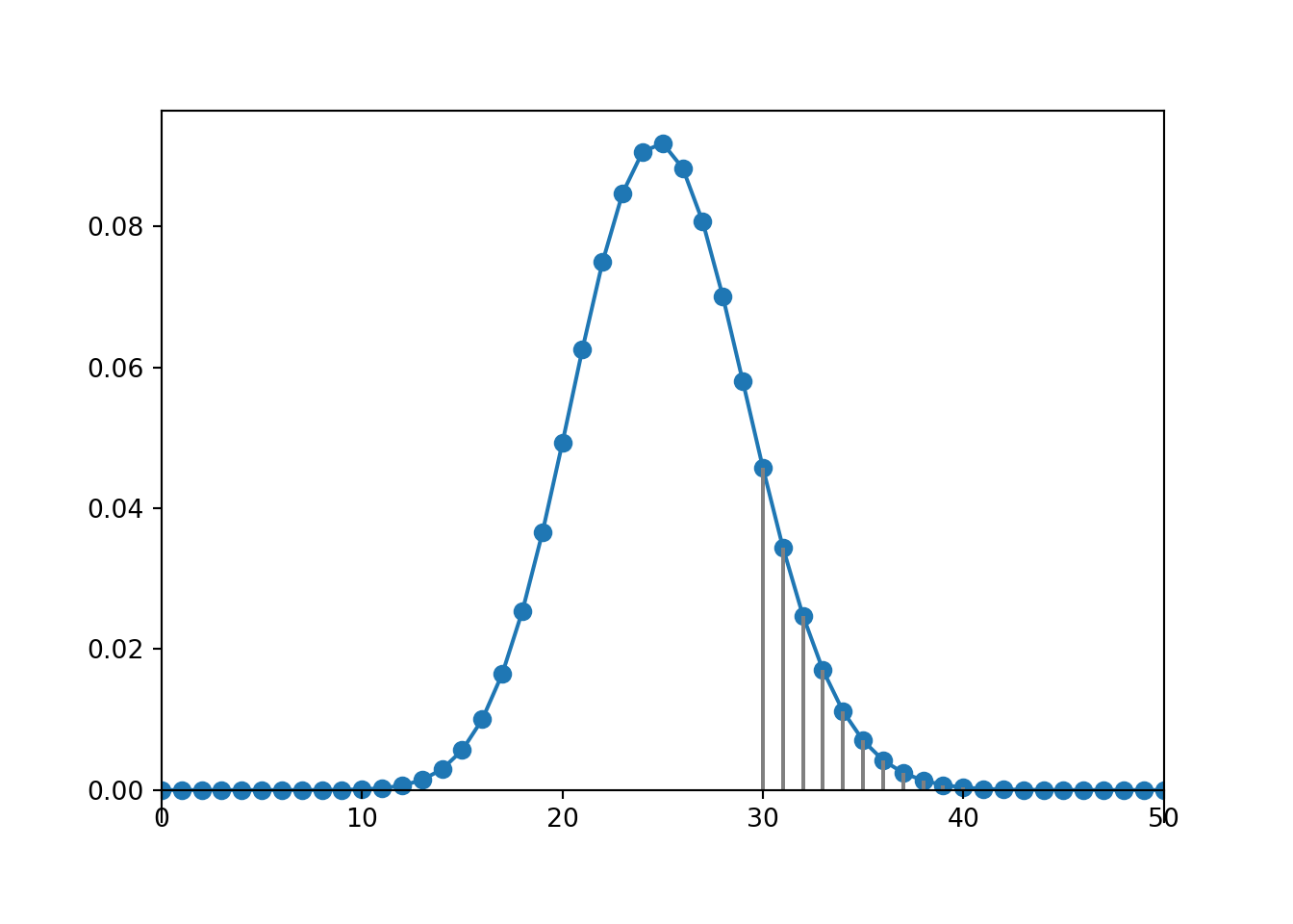
Let \(\textrm{P}\) be the probability measure which reflects that \(Roy\) has not improved. We want \(\textrm{P}(X \ge 30)=1-\textrm{P}(X<30) = 1 - \textrm{P}(X \le 29)\), where \(X\) has a Binomial(100, 0.250) distribution according to \(\textrm{P}\). In Symbulate: 1 - Binomial(100, 0.25).cdf(29) which is 0.1495. See Figure 4.9 (a)
Let \(\textrm{Q}\) be the probability measure which reflects that \(Roy\) has improved to a 0.300 hitter. We want \(\textrm{Q}(X \ge 30)=1-\textrm{Q}(X<30) = 1 - \textrm{Q}(X \le 29)\), where \(X\) has a Binomial(100, 0.300) distribution according to \(\textrm{Q}\). In Symbulate: 1 - Binomial(100, 0.30).cdf(29) which is 0.5377. See Figure 4.9 (b)
We need to decrease the probability so we want a greater (stricter) threshold than 30.
We want to find \(x\) such that \(0.01 \approx \textrm{P}(X \ge x)=1-\textrm{P}(X<x) = 1 - \textrm{P}(X \le x-1)\), where \(X\) has a Binomial(100, 0.250) distribution according to \(\textrm{P}\). Try 1 - Binomial(100, 0.25).cdf(x - 1) for different values of x to find \(x=36\), which yields \(\textrm{P}(X \ge 36)= 1 - \textrm{P}(X \le 35) = 0.009\). If the coach is only convinced if Roy gets hits in at least 36 at bats then the probability of being incorrectly convinced if Roy hasn’t improved is 0.009.
We want \(\textrm{Q}(X \ge 36)=1-\textrm{Q}(X<36) = 1 - \textrm{Q}(X \le 35)\), where \(X\) has a Binomial(100, 0.300) distribution according to \(\textrm{Q}\). In Symbulate: 1 - Binomial(100, 0.30).cdf(35) which is 0.1161. With the stricter threshold, Roy has a smaller probability of convincing the coach that he really has improved.
Now \(X\) has a Binomial(400, 0.25) distribution according to \(\textrm{P}\). Try 1 - Binomial(400, 0.25).cdf(x - 1) for different values of x to find \(x=121\), which yields \(\textrm{P}(X \ge 121)= 1 - \textrm{P}(X \le 120) = 0.01\). So if the coach is only convinced if Roy get at least 121 hits in 400 at bats then the probability of being incorrectly convinced if Roy hasn’t improved is 0.01. The probability is the same in part 4, but in part 4 Roy needed to demonstrate success in at least 36/100 = 36% of at bats, but now the threshold is 121/400 = 30.25% of at bats.
Now \(X\) has a Binomial(400, 0.30) distribution according to \(\textrm{Q}\). We want \(\textrm{Q}(X \ge 121)= 1 - \textrm{Q}(X \le 120)\), where \(X\) has a Binomial(100, 0.300) distribution according to \(\textrm{Q}\). In Symbulate: 1 - Binomial(400, 0.30).cdf(120) which is 0.4754. By demonstrating good performance over more at bats, Roy has a greater probability of convincing the coach that he really has improved.
Let \(\textrm{P}\) be the probability measure which reflects that \(Roy\) has not improved. We want \(\textrm{P}(X \ge 38)=1-\textrm{P}(X<38) = 1 - \textrm{P}(X \le 37)\), where \(X\) has a Binomial(100, 0.250) distribution according to \(\textrm{P}\). In Symbulate: 1 - Binomial(100, 0.25).cdf(37) which is 0.0027.
There are two explanations for Roy’s performance. Either Roy didn’t really improve and he just got really lucky in these 100 at bats, or he actually did improve. Since it would be so unlikely (0.0027) for Roy to get hits in at least 38 out of 100 at bats if he really hadn’t improved, the fact that he actually did this well gives us evidence that he really has improved. Did Roy necessarily improve? No. Could he have just gotten lucky? Sure. But since 38/100 would be so unlikely just by luck if he hadn’t improved, the more plausible explanation is that he actually has improved. We would say that 38/100 offers pretty convincing evidence that he has improved.
Example 4.11 featured some statistical applications of Binomial distributions, in the context of a “null hypothesis test”.
The “null hypothesis” is that Roy has not improved
A threshold like “at least 30” is a “rejection region”
The probability of exceeding the threshold if the null hypothesis is true is the probability of “Type I error” (see Figure 4.9 (a))
The probability of exceeding the threshold if Roy really has improved is the “power”, computed if \(p=0.300\), but this would generally be a function of \(p\) (see Figure 4.9 (b))
After we observe 38 hits in 100 at bats, the probability of observing a result at least that extreme if the null hypothesis is true is the “p-value”. The smaller the p-value, the stronger the evidence the observed data provides to reject the null hypothesis and conclude that Roy really has improved.
Figure 4.9: Probability of at least 30 hits in 100 at bats in Example 4.11
We will study further applications to statistics in more detail later.
In the next few examples we’ll investigate expected value and variance for Binomial distributions.
Example 4.12 Recall Example 4.1, where \(X\) had a Binomial(5, 0.25) distribution.
Suggest a “shortcut” formula for \(\textrm{E}(X)\).
Use the table from the previous part to compute \(\textrm{E}(X)\). Did the shortcut formula work?
Compute \(\textrm{P}(X = \textrm{E}(X))\).
Compute \(\textrm{P}(X \le \textrm{E}(X))\). Is it 0.5?
Interpret \(\textrm{E}(X)\) in context.
Use simulation to approximate \(\textrm{Var}(X)\) and \(\textrm{SD}(X)\).
Solution (click to expand)
Solution 4.12.
If 25% are tagged we would expect \(5(0.25) = 1.25\) tagged butterflies in the sample of 5.
Indeed we do get 1.25 if we compute the expected value the “long way” based on the distribution table. \[
(0)(0.2373) + (1)(0.3955) + (2)(0.2637) + (3)(0.0879) + (4)(0.0146) + (5)(0.0010)
\]
\(\textrm{P}(X = \textrm{E}(X)) = \textrm{P}(X = 1.25)=0\); 1.25 is not a possible value of \(X\).
\(\textrm{P}(X \le \textrm{E}(X)) = \textrm{P}(X \le 1.25)=\textrm{P}(X = 0) + \textrm{P}(X =1) = 0.2373+0.3955 = 0.633\). This is not 0.5; the distribution of \(X\) is not symmetric so the mean is not necessarily “in the middle”.
Over many samples of 5 butterflies we would expect to see 1.25 tagged butterlies per sample on average.
See simulation results below; \(\textrm{Var}(X)\) is approximately 0.9375 (we’ll see a shortcut formula for this soon) and \(\textrm{SD}(X)\) is approximately \(\sqrt{0.9375} =0.9682\).
X = RV(Binomial(5, 0.25))x = X.sim(10000)x.mean(), x.var(), x.sd()
(1.2539, 0.9474347900000001, 0.9733626199931863)
Example 4.13Figure 4.3 displays Binomial distributions for a given \(p\) (0.4) for a few different values of \(n\) (5, 10, 15, 20). As \(n\) increases does the variance increase, decrease, or stay the same?
Solution (click to expand)
Solution 4.13. For a Binomial(\(n\), \(p\)) distribution, variance increases as \(n\) increases. Since the possible values of a random variable with a Binomial distribution are \(0, 1, \ldots, n\), as \(n\) increases the range of possible values of the variable increases.
However, in some sense it is unfair to compare values from Binomial distributions with different values of \(n\). Ten successes has a very different meaning if \(n\) is 10 or 20 or 100. Rather than focusing on the absolute number of successes, in Binomial situations we are often concerned with the proportion of successes in the sample. We will see later that as the sample size \(n\) increases, the variance of the sample proportion decreases.
Example 4.14Figure 4.4 displays Binomial distributions for a given \(n\) (10) for a few different values of \(n\) (0.1, 0.3, 0.5, 0.7, 0.9).
How does the variance when \(p=0.1\) compare to when \(p=0.9\)? What about 0.3 and 0.7?
For what value of \(p\) is the variance the largest?
Among these values of \(p\), for what values of \(p\) is the variance the smallest?
What values of \(p\) (not just among those pictured) would lead to the smallest variance?
Solution (click to expand)
Solution 4.14.
The variance when \(p=0.1\) is the same as when \(p=0.9\). The shapes are mirror images (reflected about 0.5) but the degree of dispersion about the mean is the same. Moving from \(p=0.1\) to \(p=0.9\) is just like interchanging the roles of success and failure. Likewise for 0.3 and 0.7.
The distribution is most disperse, and the variance largest, when \(p=0.5\). When \(p=0.5\) we would expect the most “alterations” between success and failure in the individual trials.
Variance decreases in a symmetric manner as \(p\) moves away from 0.5. That is, variance decreases as \(p\) gets closer to 0 or 1.
The extremes \(p=0\) and \(p=1\) both result in a variance of 0. When \(p=0\), every trials results in failure so the number of successes out of \(n\) trials is always 0 and so the variance is 0. Similarly, when \(p=1\) every trials results in success so the number of successes out of \(n\) trials is always \(n\), and so the variance is 0.
The following result formalizes the observations from the last few exercises.
Lemma 4.1 If \(X\) has a Binomial(\(n\), \(p\)) distribution then
In Example 4.1, \(\textrm{Var}(X) = 5(0.25)(1-0.25) = 0.9375\), and \(\textrm{SD}(X) = \sqrt{0.9375} = 0.968\).
In Symbulate, the theoretical expected value and variance of a named distribution can be computed as Distribution(parameters).mean() and Distribution(parameters).var()
Binomial(5, 0.25).mean()
np.float64(1.25)
Binomial(5, 0.25).var()
np.float64(0.9375)
Example 4.15 Xavier bets on red on each of 3 spins of a roulette wheel. After the third spin, Xavier leaves and Zander arrives and bets on black on the next two spins. Let \(X\) be the number of bets that Xavier wins and let \(Z\) be the number that Zander wins.
Identify the distribution of \(X\) and the distribution of \(Z\).
Are \(X\) and \(Z\) independent? Explain.
What does \(X+Z\) represent in this context? Identify the distribution of \(X+Z\) without doing any calculations.
Use simulation to approximate the distribution of \(X+Z\) and confirm your answer to the previous part.
Suppose that Yolanda bets on black on all 5 spins of the wheel. Does \(X + Y\) have a Binomial distribution? Explain.
Suppose instead that Zavier bet on the number 7 in his two bets. Does \(X + Z\) have a Binomial distribution in this case? Explain.
Solution (click to expand)
Solution 4.15.
\(X\) has a Binomial(3, 18/38) distribution and \(Z\) has a Binomial(2, 18/38) distribution.
Yes, \(X\) only depends on the first three spins, and \(Z\) only depends on the last two, and the spins are (physically) independent, so \(X\) and \(Z\) are independent.
\(X+Z\) is the total number of bets won by either of these players. The five spins satisfy the Binomial situation. Each trial results in either “win” or not. The probability of a win on any bet is 18/38; it doesn’t matter if they’re betting on black or red because each has the same probability of winning. The spins are independent. Between the two players there is a fixed number of 5 bets and we are counting the number of wins. So \(X+Z\) has a Binomial(5, 18/38) distribution.
See the results below; the simulated values follow closely a Binomial(5, 13/38) distribution.
\(X + Y\) does not have a Binomial distribution, because the trials that determine \(X\) are not independent of those that determine \(Y\). The random variables \(X\) and \(Y\) are not independent.
\(X+Z\) would not have a Binomial distribution, because there is not the same probability of win (success) on all trials (18/38 for the first three but 1/38 for the last two).
Lemma 4.2 If \(X\) and \(Y\) are independent, \(X\) has a Binomial(\(n_X\), \(p\)) distribution, and \(Y\) has a Binomial(\(n_Y\), \(p\)) distribution then \(X+Y\) has a Binomial(\(n_X+n_Y\), \(p\))
A Binomial(1, \(p\)) distribution is also known as a Bernoulli(\(p\)) distribution, taking a value of 1 with probability \(p\) and 0 with probability \(1-p\). Any indicator random variable has a Bernoulli distribution.
If \(X_1, X_2, \ldots, X_n\) are independent each with a Bernoulli(\(p\)) distribution, then \(X_1+\cdots+X_n\) has a Binomial(\(n, p\)) distribution. So any random variable with a Binomial(\(n\), \(p\)) distribution has the same distributional properties as \(X_1+ X_2+ \cdots+ X_n\), where \(X_1, \ldots, X_n\) are independent each with a Bernoulli(\(p\)) distribution. This provides a very convenient representation in many problems.
Example 4.16 Continuing Example 4.1. Define the random variable \(\hat{p} = X/5\).
What does \(\hat{p}\) represent in this context. What are its possible values?
Does \(\hat{p}\) have a Binomial distribution? Does the distribution of \(\hat{p}\) have the same basic shape of a Binomial distribution?
Compute \(\textrm{P}(\hat{p} = 0.2)\).
Compute \(\textrm{E}(\hat{p})\). Why does this make sense?
Compute \(\textrm{SD}(\hat{p})\).
Suppose that 20 butterflies were selected for the second sample at random, with replacement. Compute \(\textrm{SD}(\hat{p})\); how does the value compare to the previous part?
Solution (click to expand)
Example 4.17
\(\hat{p}\) is the proportion of butterflies in the second sample that are tagged. Possible values are 0, 1/5, 2/5, 3/5, 4/5, 1.
Technically \(\hat{p}\) does not have a Binomial distribution, since a Binomial distribution always corresponds to possible values 0, 1, 2, \(\ldots, n\). But the distribution of \(\hat{p}\) does follow the same shape as the Binomial(5, 0.25) distribution, just with a rescaled variable axis.
\(\textrm{P}(\hat{p} = 0.2) = \textrm{P}(X = 1)\), which is Binomial(5, 0.25).pmf(1).
If 25% of the butterflies in the population are tagged, we would expect 25% of the butterflies in a random sample to be tagged. \[
\textrm{E}(\hat{p}) = \textrm{E}(X/5) = \textrm{E}(X)/5 = 5(0.25)/5 = 0.25
\]
The calculation is similar to the previous part. \[
\textrm{SD}(\hat{p}) = \textrm{SD}\left(\frac{X}{20}\right) = \frac{\textrm{SD}(X)}{20} = \frac{\sqrt{20(0.25)(1-0.25)}}{20} = \frac{\sqrt{0.25(1-0.25)}}{\sqrt{20}} = 0.165
\] The standard deviation of \(\hat{p}\) is smaller when \(n\) is larger. A sample of size 20 is 4 times larger than a sample of size 5, but the standard deviation is \(\sqrt{4}=2\) times smaller when \(n=20\) than when \(n=5\).
Binomial distributions model the absolute number of successes in a sample of size \(n\). If \(X\) is the number of successes then the sample proportion is the random variable \[
\hat{p} = \frac{X}{n}
\] For a fixed value of \(p\), sample-to-sample variability of \(\hat{p}\)decreases as sample size \(n\) increases. \[\begin{align*}
\textrm{E}\left(\hat{p}\right) & = p\\
\textrm{Var}\left(\hat{p}\right) & = \frac{p(1-p)}{n}\\
\textrm{SD}\left(\hat{p}\right) & = \sqrt{\frac{p(1-p)}{n}}\\
\end{align*}\]
4.6 Geometric and Negative Binomial distributions
Binomial distributions are models for the number of successes in a fixed number of Bernoulli trials. But what if the number of trials is not fixed? In particular, what if we keep performing trials until a certain number of successes are obtained?
4.6.1 Geometric distributions
Example 4.7 provided one such example, where the random variable had a Geometric distribution.
Definition 4.4 Perform Bernoulli(\(p\)) trials until a success occurs and then stop. Let \(X\) count the total number of trials, including the single success. The distribution of \(X\) is defined to be the Geometric(\(p\)) distribution.
The Geometric(\(p\)) probability mass function follows from the fact that if \(X\) has a Geometric distribution, then \(X = x\) if and only if
the first \(x-1\) trials are failures, and
the \(x\)th (last) trial results in success.
Definition 4.5 (Geometric probability mass function) A discrete random variable \(X\) has a Geometric(\(p\)) distribution if and only if its probability mass function is \[\begin{align*}
p_{X}(x) & = p (1-p)^{x-1}, & x=1, 2, 3, \ldots
\end{align*}\]
The next result follows from the fact that if \(X\) has a Geometric distribution, then \(X > x\)—that is, more than \(x\) trials are needed to achieve the first success—if and only if the first \(x\) trials result in failure.
Lemma 4.3 If \(X\) has a Geometric(\(p\)) distribution then
Example 4.18 Continuing Example 4.7, where \(X\) has a Geometric(\(p\)) distribution with \(p=0.4\).
What seems like a reasonable shortcut formula for \(\textrm{E}(X)\) in terms of \(p\)? Hint: it might help to consider the case \(p=0.1\) first, then apply similar logic to \(p=0.4\) and general \(p\).
Use Table 4.2 to compute \(\textrm{E}(X)\). Did the shortcut work?
Interpret \(\textrm{E}(X)\) in context.
Use simulation to approximate \(\textrm{E}(X)\) and \(\textrm{Var}(X)\).
Would \(\textrm{Var}(X)\) be bigger or smaller if \(p=0.9\)? If \(p=0.1\)?
Solution (click to expand)
Solution 4.16.
Suppose that she only makes 10% of her attempts, so \(p=0.1\). That is, she makes 1 in every 10 attempts on average, so it seems reasonable that we would expect her to attempt 10 three pointers on average before she makes one. Therefore, \(1/0.1= 10\) seems like a reasonable formula for \(\textrm{E}(X)\) when \(p=0.1\). In general, \(1/p\) seems like a reasonable shortcut for \(\textrm{E}(X)\) if \(X\) has a Geometric(\(p\)) distribution.
The shortcut gives \(\textrm{E}(X) = 1/0.4 = 2.5\), which is consistent with the “long way” \[
\scriptsize{
(1)(0.4) + (2)(0.24) + (3)(0.144)+(4)(0.0864) + (5)(0.0518) + (6)(0.0311) + (7)(0.0186) + (8)(0.0112) + (9)(0.0067) + \cdots
}
\] Technically, the sum keeps going but since the probabilities get so small, the contribution of the additional terms is negligible.
Imagine she does this at every practice session. Over many practice sessions, it takes her 2.5 three point attempts, until she makes one, per practice on average.
See simulation results below. We’re using the “simulate from the distribution method”.
If the probability of success is \(p=0.9\) we would not expect to wait very long until the first success, so it would be unlikely for her to need more than a few attempts. If the probability of success is \(p=0.1\) then she could make her first attempt and be done quickly, or it could take her a long time. So the variance is greater when \(p=0.1\) and less when \(p=0.9\). The probabilities in the Geometric(\(p\)) pmf decrease to 0 more quickly as \(x\) increases when \(p\) is close to 1 then when \(p\) is close to 0, so the distribution becomes “spread out” as \(p\) decreases from 1.
X = RV(Geometric(0.4))x = X.sim(10000)x.mean(), x.var(), x.sd()
In Example 4.18, \(\textrm{Var}(X) = (1-0.4)/0.4^2 = 3.75\), which is consistent with the simulation results.
If \(p=1\) then every trial results in success so \(X=1\) always and therefore the variance is 0. If \(p\) is close to 1, we expect to see success in the first few trials, so the variance is relatively small. If \(p\) is close to 0, success could occur on the first trial but we would expect to have to wait a larger number of trials until the first success occurs, resulting in a larger variance. As \(p\) gets closer to 0, the expression \((1-p)/p^2\) gets larger and larger.
You and your friend are playing the “lookaway challenge”. The game consists of possibly multiple rounds. In the first round, you point in one of four directions: up, down, left or right. At the exact same time, your friend also looks in one of those four directions. If your friend looks in the same direction you’re pointing, you win! Otherwise, you switch roles and the game continues to the next round—now your friend points in a direction and you try to look away. As long as no one wins, you keep switching off who points and who looks. The game ends, and the current “pointer” wins, whenever the “looker” looks in the same direction as the pointer.
Suppose that each player is equally likely to point/look in each of the four directions, independently from round to round.
Let \(X\) be the number of rounds played in a game.
Explain why \(X\) has a Geometric distribution, and specify the value of \(p\).
Express the event “the player who starts as the pointer wins the game” as an event involving \(X\).
Explain how you could use simulation to approximate the probability that the player who starts as the pointer wins the game and the expected number of rounds the game lasts.
Use the Geometric pmf (use software) to compute the probability that the player who starts as the pointer wins the game. Compare to the result of Example 2.50.
Compute and interpret \(\textrm{E}(X)\).
Solution (click to expand)
Solution 4.17.
\(X\) has a Geometric distribution with parameter \(p=0.25\).
Each round is a trial,
the round either results in success (current pointer wins the round and game ends) or failure (current pointer does not win the round and the game continues),
the rounds are assumed to be independent
the probability that the current point wins any particular round is 0.25
and \(X\) counts the number of rounds until the first success
The player who starts as the pointer can only win the game in odd number rounds—when they’re the pointer—so the event of interest is the event that \(X\) is odd, \(\{X \in \{1, 3, 5, 7, \ldots\}\}\).
See the code below. We could just simulate \(X\) from the Geometric(\(p\)) distribution, but we’ll use the “simulate from the probability space” method just to compare.
To simulate one round, simulate a (pointer, looker) pair of values (up, down, left, right) (or just 1, 2, 3, 4) independently, with equal probability.
If the pair of values match then the game ends in that round, otherwise the game continues
Repeat rounds as above, independently, until the game ends (the pair is a match) and then stop. Let \(X\) be the number of rounds.
Repeat the above to simulate many values of \(X\).
Average the simulated values of \(X\) to approximate \(\textrm{E}(X)\).
Count the number of simulated values of \(X\) that are odd and divide by the total number of simulated values to approximate the probability that the player who starts as the pointer wins the game.
We need to sum the Geometric(0.25) pmf over \(x=1,3,5,\ldots\). See code below. The probability is 4/7=0.571, the same as in Example 2.50
\(\textrm{E}(X) = 1/0.25 = 4\). Over many games of the lookaway challenge, the game lasts 4 rounds on average.
# given a sequence of (point, look) pairs# determine the round in which the first match occursdef count_rounds(sequence):for r, pair inenumerate(sequence):if pair[0] == pair[1]:return r +1# +1 for 0 indexing# simulate (point, look) pairs independently and equally likely# ** inf is to continue indefinitelyP = BoxModel([1, 2, 3, 4], size =2) ** infX = RV(P, count_rounds)x = X.sim(10000)x
<symbulate.distributions.Geometric object at 0x00000191AA351E50>
plt.show()
x.mean()
4.0125
The following approximate probability that the player who starts as the pointer wins the game (which occurs if the game ends in an odd number of rounds).
def is_odd(u):return (u %2) ==1# odd if the remainder when dividing by 2 is 1x.count(is_odd) / x.count()
0.5649
We can find the theoretical probability that \(X\) is odd by summing the Geometric(0.25) pmf over \(x = 1, 3, 5, \ldots\). Technically, the sum keeps going but the probabilities get extremely small as \(x\) increases, so we just cut it off after some large value (99 below).
# range(1, 100, 2) is odd numbers from 1 to 99Geometric(0.25).pmf(range(1, 100, 2)).sum()
np.float64(0.5714285714283882)
4.6.2 Negative Binomial distributions
Now we’ll investigate a generalization of the Geometric situation where we perform Bernoulli trials until a certain number (not necessarily one) of successes are obtained.
Example 4.20 Maya is a basketball player who makes 86% of her free throw attempts. Suppose that she attempts free throws until she makes 5 and then stops. Let \(X\) be the total number of free throws she attempts. Assume shot attempts are independent.
Does \(X\) have a Binomial distribution? A Geometric distribution? Why or why not?
What are the possible values of \(X\)? Is \(X\) discrete or continuous?
Describe how you could use a tactile simulation to simulate a single value of \(X\).
Describe in words how you could use simulation to approximate \(\textrm{P}(X=5)\).
Describe in words how you could use simulation to approximate the distribution of \(X\).
Write and run Symbulate code to approximate \(\textrm{P}(X=5)\) and the distribution of \(X\).
Compute the theoretical value of \(\textrm{P}(X = 5)\). Compare to your simulated value. Is the theoretical value within the margin of error of the simulated value?
Interpret in context \(\textrm{P}(X = 5)\) as a long run relative frequency.
The distribution of \(X\) is called the “NegativeBinomial(5, 0.86)” distribution. Use Symbulate to compute \(\textrm{P}(X = x\) for all possible values \(x\), then construct a table, plot, and spinner representing the approximate distribution of \(X\). (You can cut it off after the probabilities get very small.) Are the simulation results consistent with the theoretical distribution?
What seems like a reasonable shortcut formula for \(\textrm{E}(X)\)?
Use the theoretical pmf to compute \(\textrm{E}(X)\). Did the shortcut formula work.
Interpret \(\textrm{E}(X)\) for this example.
Would the variance be larger or smaller if attempted free throws until she made 10 instead of 5?
Solution (click to expand)
Solution 4.18.
\(X\) does not have a Binomial distribution since the number of trials is not fixed. The number of successes is fixed to be 5, but the number of trials is random. \(X\) also does not have a Geometric distribution because \(X\) counts the number of trials needed for 5 successes, not just one.
\(X\) can take values 5, 6, 7, \(\ldots\). Even though it is unlikely that \(X\) is very large, there is no fixed upper bound. Even though \(X\) can take infinitely values, \(X\) is a discrete random variables because it takes countably many possible values.
Construct a spinner that lands on success with probability 0.86. Spin the spinner until it lands on 5 successes and stop and count the total number of spins; this is one simulated value of \(X\).
Simulate many values of \(X\) as in the previous part. Count the number of simulated values equal to 5 and divide by the total number of simulated values to approximate \(\textrm{P}(X=5)\).
Simulate many values of \(X\) and summarize the simulated values to find the simulated relative frequency for each possible value.
See code below.
In order for \(X\) to be 5, Maya must make her first 5 attempts. Since the attempts are independent \(\textrm{P}(X=5)=(0.86)^5=0.47\), which is consistent with the simulation results.
If Maya does this every practice, then in about 47% of practices she will make her first five free throw attempts.
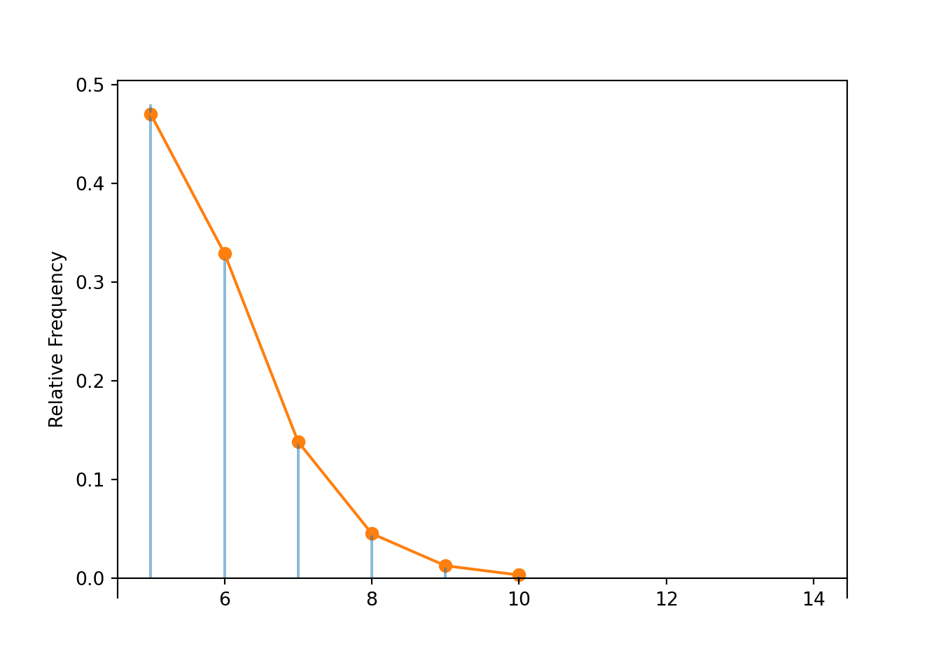
See the Symbulate code below and Table 4.3 and Table 4.3. The simulation results are consistent with the theoretical distribution.
On average it takes \(1/0.86 = 1.163\) attempts to make a free throw, so it seems reasonable that it would take on average \(5(1/0.86)=5.81\) attempts to make 5 free throws.
The shortcut gives \(\textrm{E}(X) = 5(1/0.86)=5.81\), which is consistent with the “long way” \[
\scriptsize{
(5)(0.4705) + (6)(0.3293) + (7)(0.1383)+(8)(0.0452) + (9)(0.0127) + (10)(0.0032) + (11)(0.0007) + \cdots
}
\] Technically, the sum keeps going but since the probabilities get so small, the contribution of the additional terms is negligible.
If Maya does this at every practice, it takes her on average 5.8 attempts to make 5 free throws.
The variance would be larger with 10 attempts. With every additional required success we “accumulate variability” in the total number of attempts needed to achieve that many successes.
r =5def count_until_rth_success(omega): trials_so_far = []for i, w inenumerate(omega): trials_so_far.append(w)ifsum(trials_so_far) == r:return i +1# +1 for zero-based indexing# simulate an indefinite (** inf) sequence of Bernoulli trials P = Bernoulli(0.86) ** infX = RV(P, count_until_rth_success)x = X.sim(10000)x.plot()# overlay theretical distributionNegativeBinomial(r =5, p =0.86).plot();plt.show()
x.count_eq(7) /10000
0.1372
x.mean()
5.7961
x.var()
0.9377247899999999
We can use Symbulate to compute theoretical Negative Binomial probabilities.
The values \(5, \ldots, 11\) account for 99.98% of the probability: \(\textrm{P}(X \le 11) = 0.9998\)
NegativeBinomial(5, 0.86).cdf(11)
np.float64(0.999793358732864)
NegativeBinomial(5, 0.86).mean()
np.float64(5.813953488372093)
NegativeBinomial(5, 0.86).var()
np.float64(0.946457544618713)
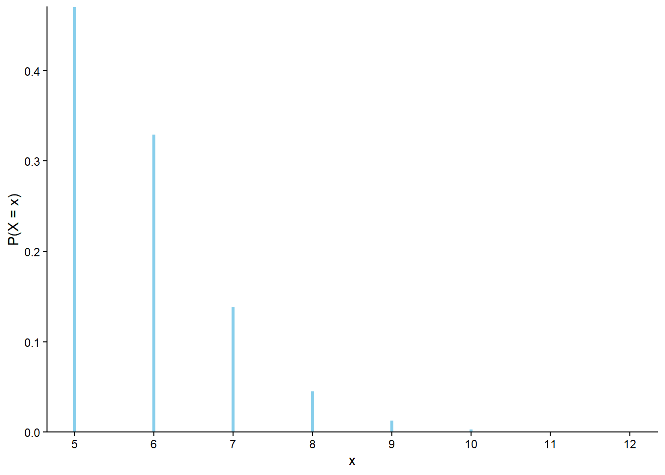
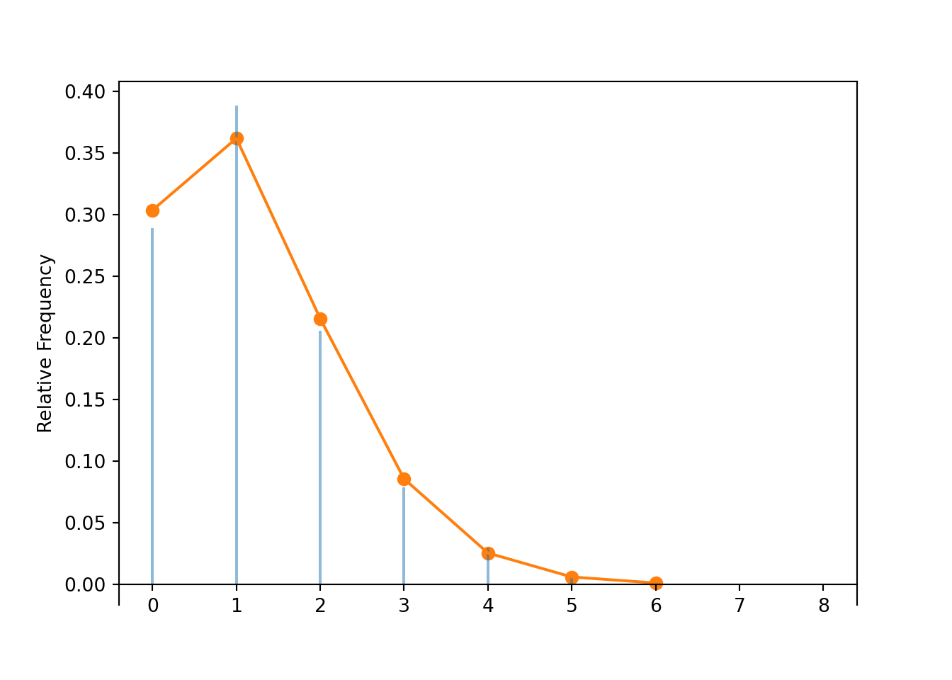
Table 4.3: Table representing the the NegativeBinomial(5, 0.86) distribution, the theoretical distribution of \(X\) in Example 4.20.
x
P(X = x)
5
0.4704
6
0.3293
7
0.1383
8
0.0452
9
0.0127
10
0.0032
11
0.0007
12
0.0002
(a) Impulse plot
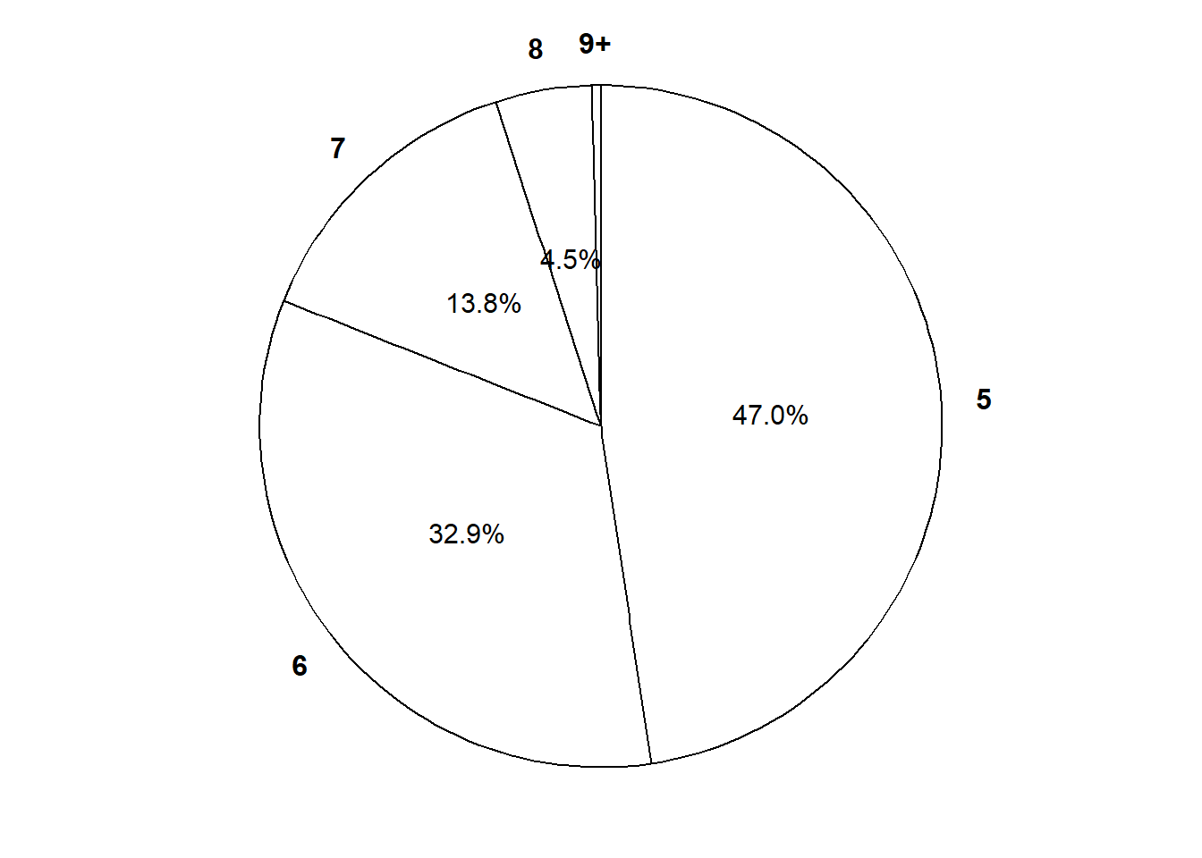
(b) Spinner; the values 9 and up have been grouped together and their total probability of 1.7% is not displayed.
Figure 4.10: Plot and spinner representing the the NegativeBinomial(5, 0.86) distribution, the theoretical distribution of \(X\) in Example 4.20.
Definition 4.6 Perform Bernoulli(\(p\)) trials until a fixed number, \(r\), of successes and then stop. Let \(X\) count the total number of trials, including the \(r\) successes. The distribution of \(X\) is defined to be the Negative Binomial(\(r\), \(p\)) distribution.
A Negative Binomial distribution is specified by two parameters:
\(r\) (an integer): the fixed number of successes
\(p\) (in \([0, 1]\)): the fixed marginal probability of success on each Bernoulli trial, or the population proportion of success
Lemma 4.5 If \(X\) has a NegativeBinomial(\(r\), \(p\)) distribution \[\begin{align*}
\textrm{E}(X) & = \frac{r}{p}\\
\textrm{Var}(X) & = \frac{r(1-p)}{p^2}
\end{align*}\]
Example 4.21 What is another name for a NegativeBinomial(1, \(p\)) distribution?
Solution (click to expand)
Solution 4.19. A NegativeBinomial(1, \(p\)) distribution is a Geometric(\(p\)) distribution.
Example 4.22 Xavier bets on red on roulette until he wins 3 bets and then he leaves. After Xavier leaves, Zander arrives and bets on black until he wins 2 bets and then he leaves. Let \(X\) be the number of bets that Xavier makes and let \(Z\) be the number of bets that Zander makes.
Identify the distribution of \(X\) and the distribution of \(Z\).
Are \(X\) and \(Z\) independent? Explain.
What does \(X+Z\) represent in this context? Identify the distribution of \(X+Z\) without doing any calculations.
Use simulation to approximate the distribution of \(X+Z\) and confirm your answer to the previous part.
Suppose that Yolanda starts making bets on the same game as Xavier, and she bets on black until she wins 5 bets. Does \(X + Y\) have a Negative Binomial distribution? Explain.
Suppose instead that Zavier bets on the number 7 until he wins 5 bets. Does \(X + Z\) have a Negative Binomial distribution in this case? Explain.
Solution (click to expand)
Solution 4.20.
\(X\) has a NegativeBinomial(3, 18/38) distribution and \(Z\) has a NegativeBinomial(2, 18/38) distribution.
Yes, Xavier and Zander bet on different sets of games and the spins are (physically) independent, so \(X\) and \(Z\) are independent.
\(X+Z\) is the total number of games played until a total of 5 games are won. This satisfies the Negative Binomial situation. Each trial results in either “win” or not. The probability of a win on any bet is 18/38; it doesn’t matter if they’re betting on black or red because each has the same probability of winning. The spins are independent. Between the two players there is a fixed number of 5 wins and we are counting the total number of bets (trials). So \(X+Z\) has a NegativeBinomial(5, 18/38) distribution.
See the results below; the simulated values follow closely a NegativeBinomial(5, 18/38) distribution.
\(X + Y\) does not have a Negative Binomial distribution, because the trials that determine \(X\) are not independent of those that determine \(Y\). The random variables \(X\) and \(Y\) are not independent.
\(X+Z\) would not have a Negative Binomial distribution, because there is not the same probability of win (success) on all trials (18/38 for Xavier’s bets but 1/38 for Zander’s).
Lemma 4.6 If \(X\) and \(Y\) are independent, \(X\) has a NegativeBinomial(\(r_X\), \(p\)) distribution, and \(Y\) has a NegativeBinomial(\(r_Y\), \(p\)) distribution then \(X+Y\) has a NegativeBinomial(\(r_X+r_Y\), \(p\))
If \(X_1, X_2, \ldots, X_r\) are independent each with a Geometric(\(p\)) distribution, then \(X_1+\cdots+X_r\) has a NegativeBinomial(\(r, p\)) distribution. So any random variable with a NegativeBinomial(\(r\), \(p\)) distribution has the same distributional properties as \(X_1+ X_2+ \cdots+ X_r\), where \(X_1, \ldots, X_r\) are independent each with a Geometric(\(p\)) distribution. This provides a very convenient representation in many problems.
4.6.3 Pascal distributions
In a Negative Binomial situation, the total number of successes is fixed (\(r\)), i.e., not random. What is random is the number of failures, and hence the total number of trials.
Our definition of a Negative Binomial distribution (and hence a Geometric distribution) provides a model for a random variable which counts the number of Bernoulli(\(p\)) trials required until \(r\) successes occur, including the \(r\) trials on which success occurs, so the possible values are \(r, r+1, r+2,\ldots\)
There is an alternative definition of a Negative Binomial distribution (and hence a Geometric distribution) which provides a model for a random variable which counts the number of failures in Bernoulli(\(p\)) trials required until \(r\) successes occur, excluding the \(r\) trials on which success occurs, so the possible values are \(0, 1, 2, \ldots\) We will refer to this alternative definition as a “Pascal distribution”.
Definition 4.7 Perform Bernoulli(\(p\)) trials until a fixed number, \(r\), of successes and then stop. Let \(X\) count the total number of failures (excluding the \(r\) successes). The distribution of \(X\) is defined to be the Pascal(\(r\), \(p\)) distribution.
There is not a standard definition of Negative Binomial, and some software programs use “Negative Binomial” to refer to what we’re calling “Pascal”. It’s a good idea to always check the documentation of a software package to see what definition is used.
In Symbulate, a Pascal(\(r\), \(p\)) distribution follows this alternate definition. In Symbulate,
The possible values of a NegativeBinomial(\(r\), \(p\)) distribution are \(r, r+1, r+2,\ldots\)
The possible values of a Pascal(\(r\), \(p\)) distribution are \(0, 1, 2,\ldots\)
If \(X\) has a NegativeBinomial(\(r\), \(p\)) distribution then \((X-r)\) has a Pascal(\(r\), \(p\)) distribution. Similarly, if \(Y\) has a Pascal(\(r\), \(p\)) distribution then \((Y+r)\) has a NegativeBinomial(\(r\), \(p\)) distribution.
4.7 Poisson distributions
Binomial and Negative Binomial distributions are commonly used for modeling discrete random variables. However, Binomial and Negative Binomial models are not appropriate in many situations that involve counting “successes”.
Example 4.23 Let \(X\) be the number of home runs hit (in total by both teams) in a randomly selected Major League Baseball game.
In what ways is this situation like the Binomial situation? (What is a trial? What is “success”?)
In what ways is this NOT like the Binomial situation?
Solution (click to expand)
Solution 4.21.
Each pitch is a trial, and on each trial either a home run is hit (“success”) or not. The random variable \(X\) counts the number of home runs (successes) over all the trials
Even though \(X\) is counting successes, this is not the Binomial situation.
The number of trials is not fixed. The total number of pitches varies from game to game. (The average is around 300 pitches per game).
The probability of success is not the same on each trial. Different batters have different probabilities of hitting home runs. Also, different pitch counts or game situations lead to different probabilities of home runs.
The trials might not be independent. Make sure you distinguish independence from the previous assumption of unequal probabilities of success; you need to consider conditional probabilities to assess independence. Maybe if a pitcher gives up a home run on one pitch, then the pitcher is “rattled” so the probability that he also gives up a home run on the next pitch increases, or the pitcher gets pulled for a new pitcher which changes the probability of a home run on the next pitch.
Example 4.24 Let \(X\) be the number of vehicle crashes involving fatalities that occur in San Luis Obispo County in a randomly selected week.
In what ways is this like the Binomial situation? (What is a trial? What is “success”?)
In what ways is this NOT like the Binomial situation?
Which of the following do you think it would be easier to estimate by collecting and analyzing relevant data?
The total number of vehicles on the road in the county in a week, and the probability that each vehicle is involved in a fatal crash.
The average number of fatal vehicle crashes per week in the county.
Solution (click to expand)
Solution 4.22.
Each vehicle on the road in the week is a trial, and each vehicle either is either involved in a fatal crash (“success”) or not. The random variable \(X\) counts the number of vehicles involved in fatal crashes (successes). (Remember “success” is just a generic label for what you’re interested in counting; “success” is not necessarily good.)
Even though \(X\) is counting successes, this is not the Binomial situation.
The number of trials is not fixed. The total number of vehicles on the road varies from week to week.
The probability of success is not the same on each trial. Different drivers have different probabilities of being involved in fatal crashes; some drivers are safer than others. Also, different conditions increase the probability of a crash, like driving at night.
The trials are plausibly not independent. Make sure you distinguish independence from the previous assumption of unequal probabilities of success; you need to consider conditional probabilities to assess independence. If a vehicle is in a crash, then the probability of being involved in a crash increases for the vehicles that are driving near it.
It would be extremely difficult to estimate the probability that each individual vehicle is involved in a fatal crash. You might be able to measure the total number of vehicles in a week at a certain location (e.g., with cables across the road), but doing so for the entire county would be extremely difficult, and it vary from week to week. It would be much easier to find data on total number of fatal vehicle crashes in a week, e.g., from police reports, and use it to estimate the average number of fatal vehicle crashes per week in the county. That is, you could count the number of “successes” without knowing how many “trials” there were or the probability of “success” on individual trials.
Binomial and Negative Binomial models have several restrictive assumptions that might not be satisfied in practice:
The number of trials must be fixed (not random) and known (for Negative Binomial, the number of successes must be fixed)
The probability of success must be the same for each trial (fixed, not random) and known.
The trials must be independent.
Even when the trials are independent with the same probability of success, fitting a Binomial model to data requires estimation of both \(n\) and \(p\) individually. When the only data available are counts of successes but not trials (e.g., number of fatal vehicle crashes in a week but not number of vehicles) it might not be possible to estimate both \(n\) and \(p\).
“Poisson models” are more flexible models for counts which do not require all the conditions of the Binomial situation. Poisson distributions are often used to model the distribution of random variables that count the number of “relatively rare” events that occur over a certain interval of time or in a certain region (e.g., number of car insurance policies that have claims in a day, number of bank loans that go into default, number of mutations in a DNA sequence, number of earthquakes that occurs in SoCal in an hour, etc.)
Example 4.25 Recall our discussion of the matching problem in Section 3.13. We observed that, unless \(n\) is really small,
the long run average number of matches does is (approximately) 1
the distribution of the number of matches (\(X\)) is approximately the “Poisson(1)” distribution.
Interpret \(\textrm{P}(X = 0)\) as a long run relative frequency.
Describe in words the Poisson(1) distribution. What are some relevant features? Which values are most likely? How much more likely are they than the next most likely value? And so on.
Would it be appropriate to assume that \(X\) has a Binomial distribution? Explain.
Solution (click to expand)
Solution 4.23.
In about 37% of repetitions of the matching problem, there will be no matches. For example, in about 37% of Secret Santa drawings, no one will draw their own name.
We could interpret the distribution in terms of relative frequencies as in the previous part: 18.4% of repetitions of the matching problem result in exactly 2 matches, etc. We can also interpret the distribution in terms of relative degrees of likelihood.
0 and 1 are equally likely, and then the pmf is decreasing as a function of \(x\)
2 is 1/2 as likely as 1
3 is 1/3 as likely as 2,
4 is 1/4 as likely as 3
5 is 1/5 as likely as 4, and so on
In some ways the matching problem does resemble the Binomial situation:
Each object is a trial and success occurs if it is put in the correct spot.
There are \(n\) trials, fixed.
Unconditionally, each object is equally likely to be placed in any of the \(n\) spots, so the marginal probability of success is the same on each trial, \(1/n\).
\(X\) counts the number of successes in \(n\) trials.
However, the trials are not independent. For example, if object 1 is placed correctly in spot 1, the conditional probability that object 2 is placed in spot 2 is \(1/(n-1)\); if objects 1 through \(n-1\) are placed in their correct spots, then the conditional probability that object \(n\) is placed in the correct spot is 1. Since the trials are not independent, \(X\) does not have a Binomial distribution.
A Poisson distribution has a single parameter, denoted \(\mu\), which must be a positive number, \(\mu > 0\). One way to interpret \(\mu\) is as the expected value, that is, long run average value. In the matching problem 1 is the parameter of the Poisson distribution because 1 is the long run average number of matches. Figure 4.11 displays Poisson distributions for a few values of \(\mu\).
mus = [0.7, 1.6, 2.5, 3.4]plt.figure();for mu in mus: Poisson(mu).plot();plt.show()
Figure 4.11: Probability mass functions of Poisson distributions; \(\mu\) values, from left to right, 0.7, 1.6, 2.5, 3.4.
Example 4.25 and Figure 4.11 illustrate the “Poisson pattern”. As a function of \(x=0, 1, 2, \ldots\), a Poisson(\(\mu\)) pmf increases for \(x<\mu\) and then decreases4 for \(x>\mu\), following a particular Poisson pattern:
1 is \(\mu\) times as likely as 0
2 is \(\mu/2\) times as likely as 1
3 is \(\mu/3\) times as likely as 2
4 is \(\mu/4\) times as likely as 3
and so on.
Definition 4.8 A random variable \(X\) has a Poisson(\(\mu\)) distribution if the possible values are \(0, 1, 2, \ldots\) and the pmf follows the
\[
\text{Poisson(}\mu\text{) pattern:}\quad x \text{ is } \frac{\mu}{x} \text{ as likely as } x-1 \quad \text{ (for } x = 1, 2, 3, \ldots)
\]
The Poisson pattern is sufficient to define the shape of a Poisson(\(\mu\)) pmf \(p(x), x = 0, 1, 2, \ldots\). The final step is to normalize the probabilities defined by the Poisson pattern so that they sum to 1.
For example, for the Poisson(1) distribution in Example 4.25 suppose that 0 accounts for 10000 “units” of probability; remember, this is just an arbitrary baseline. Then the Poisson pattern implies that
0 accounts for \(10000\) units (just an assumed baseline)
1 accounts for \(10000\times 1/1 = 10000\) units
2 accounts for \(10000\times 1/2 = 5000\) units
3 accounts for \(5000\times 1/3 = 1666.67\) units
4 accounts for \(1666.67\times 1/4 = 416.67\) units
5 accounts for \(416.67\times 1/5 = 83.33\) units
6 accounts for \(83.33\times 1/6 = 13.89\) units
7 accounts for \(13.89\times 1/7 = 1.98\) units
And so on. Technically, a Poisson(1) distribution assigns positive probability to all whole numbers, but the values \(0,\ldots,7\) comprise nearly 100% of the probability. The values \(0,\ldots,7\) account for a total of 27182.82 “units”, so we divide the units corresponding to each of \(0,\ldots,7\) by 27182.82 to obtain probabilities which sum to 1, resulting in the values in Table 3.18 (e.g., the value 3 corresponds to probability \(1666.67 / 27182.82 = 0.0613\)). Note that, after normalizing, the value 0 corresponds to probability \(e^{-1} = 0.3679\).
If \(X\) has a Poisson(\(\mu\)) distribution, normalization implies that5 the probability that \(X\) equals 0 is \(e^{-\mu}\). This fact provides a baseline for computing other probabilities via the Poisson pattern without dealing with arbitrary “units”6.
Example 4.26 Let \(X\) be the number of home runs hit (in total by both teams) in a randomly selected Major League Baseball game. Assume that \(X\) has a Poisson(2.4) distribution.
In what sense are home runs “relatively rare”?
What are the possible values of \(X\)?
Interpret the parameter 2.4 in context.
Compute \(\textrm{P}(X = 2.4)\) without using software.
Identify the most likely value of \(X\) without doing any computations.
Use Symbulate to compute \(\textrm{P}(X = 0)\) and interpret the value in context.
Starting with \(\textrm{P}(X = 0)\) from the previous part, use the “Poisson pattern” to find, by hand without Symbulate, \(\textrm{P}(X = x)\) for \(x = 1, 2, 3, 4, \ldots\). Then use Symbulate to check your values, and display them in a table and plot.
Use Symbulate to simulate many values of \(X\) and compare the simulated distribution to the theoretical Poisson distribution and its expected value and variance.
Solution (click to expand)
Solution 4.24.
In a typical baseball game there are around 300 pitches but only a handful of home runs. So home runs (successes) are rare relative to the number of pitches (trials).
Since \(X\) has a Poisson distribution, its possible values are \(0, 1, 2, \ldots\) Even though it is rare for a game to have more than a few home runs (see below), technically there is no fixed upper bound for the number of home runs that can happen in a game.
2.4 is the long run average value of \(X\): Over many baseball games there are a total of 2.4 home runs per game on average.
\(\textrm{P}(X = 2.4) = 0\) since 2.4 is not a possible value of \(X\). The long run average is 2.4, but the number of home runs in any game must be a whole number.
As a function of \(x\) a Poisson pmf increases up to \(\mu\) and then decreases, so with \(\mu = 2.4\) the value \(x=2\) will have the highest probability.
We can use Poisson(2.4).pmf(0) to obtain \(\textrm{P}(X = 0) = 0.091\). (We could also use the Poisson normalizing constant: \(\textrm{P}(X = 0)=e^{-2.4} = 0.091\).) Over many baseball games, about 9.1% of games have 0 home runs, so about 89.9% of games have at least one home run. In other words, a baseball game is about 10 times more likely to have at least one home run than to have 0 home runs.
Just sum the values of the pmf corresponding to the values \(x = 0, 1, \ldots, 13\): \(\textrm{P}(X \le 13) = 0.9999997\). There isn’t any shorter way to do it. In the long run, almost all MLB games have at most 13 home runs. Even though the Poisson(2.4) pmf assigns nonzero probability to all whole numbers 0, 1, 2, \(\ldots\), the probability that \(X\) takes a value greater than 13 is extremely small.
See Figure 4.12 (b). To simplify the display we have lumped values \(6, 7, \ldots\) into one “6+” category.
Compute the probability-weighted average to find \(\textrm{E}(X)=2.4\). \[
\scriptsize{
(0)(0.0907)+(1)(0.2177)+(2)(0.2613)+(3)(0.2090)+(4)(0.1254)+(5)(0.0602)+(6)(0.0241)+(7)(0.0083)+(8)(0.0025)+(9)(0.0007)+\cdots
}
\] Technically the sum would keep going but since the probabilities get so small the contribution of the remaining terms is negligible.
Compute \(\textrm{E}(X^2)=8.16\). \[
\scriptsize{
(0^2)(0.0907)+(1^2)(0.2177)+(2^2)(0.2613)+(3^2)(0.2090)+(4^2)(0.1254)+(5^2)(0.0602)+(6^2)(0.0241)+(7^2)(0.0083)+(8^2)(0.0025)+(9^2)(0.0007)+\cdots
}
\] Technically the sum would keep going but since the probabilities get so small the contribution of the remaining terms is negligible. Then \(\textrm{Var}(X) = \textrm{E}(X^2)- (\textrm{E}(X))^2 = 8.16 - 2.4^2 = 2.4\)
See the simulation results below, which match up closely with the theoretical distribution.
(a) Impulse plot
(b) Spinner; the values 6, 7,… have been grouped together and their total probability of 3.6% is not displayed.
Figure 4.12: Plot and spinner representing the the Poisson(2.4) distribution, the theoretical distribution of \(X\) in Example 4.26.
Since Poisson is a named distribution family in Symbulate, we can use pmf to compute probabilities such as \(\textrm{P}(X = 0)\), \(\textrm{P}(X = x)\) for \(x = 0, 1, 2, \ldots\), and \(\textrm{P}(X \le 13)\).
Poisson(2.4).pmf(0)
np.float64(0.09071795328941251)
xs =list(range(13+1))pmf_x = [Poisson(2.4).pmf(x) for x in xs]print(tabulate({'x': xs,'Poisson(2.4) pmf(x)': pmf_x}, headers ='keys', floatfmt=".4f"))
Now for a simulation. We define a Symbulate RV by specifying its distribution; this basically tells Symbulate to use the spinner in Figure 4.12 (b) to simulate values of \(X\).
X = RV(Poisson(2.4))
Now we simulate many values; note that each simulated value is a whole number.
x = X.sim(10000)x
Index
Result
0
0
1
1
2
0
3
2
4
2
5
4
6
2
7
3
8
1
...
...
9999
3
Finally, we summarize the simulated values. The average of many simulated values is close to the long run average of 2.4.
x.mean()
2.4073
x.var()
2.39640671
We can summarize the simulated values to approximate the distribution of \(X\). Since we defined \(X\) by specifying its Poisson(2.4) distribution, we’re basically just verifying that the simulation is doing what we told it to do.
x.tabulate(normalize =True)
Value
Relative Frequency
0
0.0901
1
0.2148
2
0.2636
3
0.2084
4
0.1267
5
0.0614
6
0.0236
7
0.0076
8
0.003
9
0.0005
10
0.0003
Total
1.0
plt.figure();x.plot();# Plot the simulated values Poisson(2.4).plot();# Plot the theoretical pmf
<symbulate.distributions.Poisson object at 0x00000191AA44F950>
plt.show();
In Example 4.26 we assumed that the number of home runs per game follows a Poisson(2.4) distribution. Is this reasonable? Table 4.4 summarizes home run data7 from all regular season MLB games in the 2023 season. There were 5868 home runs in 2430 games, an average of 2.4 home runs per game. The observed relative frequencies are pretty close to the theoretical Poisson(2.4) probabilities; see Figure 4.13 for a visual comparison. We can see that the Poisson(2.4) distribution models the number of home runs per game reasonably well, at least based on the 2023 data.
Table 4.4: Data on home runs per game in the 2023 MLB season, compared with the Poisson(2.4) distribution.
Number of HRs
Number of games
Proportion of games
Poisson probability
0
244
0.1004
0.0907
1
559
0.2300
0.2177
2
597
0.2457
0.2613
3
479
0.1971
0.2090
4
288
0.1185
0.1254
5
141
0.0580
0.0602
6
68
0.0280
0.0241
7
27
0.0111
0.0083
8
21
0.0086
0.0025
9
5
0.0021
0.0007
10
0
0.0000
0.0002
11
1
0.0004
0.0000
12
0
0.0000
0.0000
Total
2430
1.0000
1.0000
Figure 4.13: Home runs per game in MLB games. Blue spikes represent observed relative frequencies from 2023 season data. Orange dots represent the Poisson(2.4) pmf.
A Poisson distribution is a discrete distribution which assign nonzero probability to countably infinitely many values: \(0, 1, 2, \ldots\). While there is no fixed upper bound, for many Poisson distributions most of the probability is concentrated over a relatively small range of possible values.
Poisson distributions are often reasonable models for random variables which count successes in situations where successes are rare relative to the number of trials. In Example 4.24, there are many vehicles on the road but very few of them are involved in fatal crashes. Therefore, if \(X\) is the number of vehicles crashes involving fatalities that occur in San Luis Obispo County in a randomly selected week, we might assume that \(X\) follows a Poisson distribution. We could estimate the parameter by collecting data on the number of fatal vehicle crashes in a sample of weeks and computing the average number of fatal crashes per week. Table 4.5 summarizes such data8 for 2011 through 2020 from San Luis Obispo County. There were 277 fatal vehicle crashes in 519 weeks, an average of 0.53 fatal vehicle crashes per week. The observed relative frequencies in Table 4.5 are pretty close to the theoretical Poisson(0.53) probabilities; see also Figure 4.14.
Table 4.5: Data on weekly fatal vehicle crashes in San Luis Obispo County 2011-2020, compared with the Poisson(0.53) distribution.
Number of fatal crashes
Number of weeks
Proportion of weeks
Poisson probability
0
300
0.5780
0.5864
1
168
0.3237
0.3130
2
45
0.0867
0.0835
3
5
0.0096
0.0149
4
1
0.0019
0.0020
5
0
0.0000
0.0002
Total
519
1.0000
1.0000
Figure 4.14: Weekly fatal vehicle crashes in San Luis Obispo County. Blue spikes represent observed relative frequencies based on 2011-2020 data. Orange dots represent the Poisson(0.53) pmf.
We have seen two data sets that provide some motivation for the Poisson pattern, and there are many other examples. Why is the Poisson pattern so ubiquitous? Later we will explore more deeply the theory and properties of Poisson distributions. For now just remember that Poisson distributions are one of the most commonly used probability models for discrete random variables, especially when counting “relatively rare” events.
Example 4.27Figure 4.11 displays Poisson(\(\mu\)) pmfs for a few values of \(\mu\). As \(\mu\) increases, does the variance increases, decrease, or stay the same?
Solution (click to expand)
Solution 4.25. As \(\mu\) increases, the variance increases. For Poisson(\(\mu\)) pmf \(p(x)\)
\(p(x)\) increases for \(x<\mu\): \(\frac{p(x)}{p(x-1)} = \frac{\mu}{x}>1\) if \(x<\mu\). The larger \(\mu\) is, the longer and slower the probabilities increase for \(x<\mu\).
\(p(x)\) decreases for \(x>\mu\): \(\frac{p(x)}{p(x-1)} = \frac{\mu}{x}<1\) if \(x>\mu\). The larger \(\mu\) is, the longer and slower the probabilities decrease for \(x>\mu\).
It wasn’t a coincidence in Example 4.26 that both \(\textrm{E}(X)\) and \(\textrm{Var}(X)\) were equal to 2.4.
Lemma 4.7 If \(X\) has a Poisson(\(\mu\)) distribution then
For a Poisson distribution, both the mean and variance are equal to \(\mu\), but remember that the mean is measured in the count units (e.g., home runs) but the variance is measured in squared units (e.g., \(\text{(home runs)}^2\)).
4.7.1 Poisson aggregration
Table 4.5 showed that the number of fatal crashes in each week in SLO County followed, approximately, the Poisson pattern. What if instead we had looked at crashes in each month or each year?
Example 4.28 Suppose that the number of fatal crashes in SLO County in a week follows, approximately, a Poisson(0.53) distribution, independently from week to week. Let \(X\) be the number of fatal crashes in a period of 4 consecutive weeks (close enough to a “month”).
How could you use a spinner to simulate a value of \(X\)?
What is \(\textrm{E}(X)\)? You should be able to compute it without knowing the distribution of \(X\).
Use simulation to approximate the distribution of \(X\). Does the approximate distribution follow (approximately) the Poisson pattern?
Solution (click to expand)
Solution 4.26.
Construct a spinner corresponding to Poisson(0.53) distribution; see Table 4.5. Spin the spinner 4 times and sum the values; this is one value of \(X\).
\(\textrm{E}(X) = 4(0.53)=2.12\). If there are 0.53 accidents per week on average, there are 2.12 accidents per 4-week period on average.
See simulation results below. The simulated distribution of \(X\) does roughly follow the Poisson pattern with \(\mu = 2.12\).
P = Poisson(0.53) **4X = RV(P, sum)(RV(P) & X).sim(10)
Example 4.28 is an example of “Poisson aggregation”.
Lemma 4.8 (Poisson aggregation) If \(X\) and \(Y\) are independent, \(X\) has a Poisson(\(\mu_X\)) distribution, and \(Y\) has a Poisson(\(\mu_Y\)) distribution, then \(X+Y\) has a Poisson(\(\mu_X+\mu_Y\)) distribution.
If \(X\) has mean \(\mu_X\) and \(Y\) has mean \(\mu_Y\) then linearity of expected value implies that \(X+Y\) has mean \(\mu_X + \mu_Y\). What Poisson aggregation says is that if component counts are independent and each follows a Poisson pattern, then the total count also follows a Poisson pattern.
4.7.2 Poisson paradigm
This section will provide some background on why the Poisson pattern is so ubiquitous.
Example 4.29 Suppose that the number of typographical errors on a randomly selected page of a textbook has a Poisson distribution with parameter \(\mu = 0.3\).
Find the probability that a randomly selected page has no typographical errors.
Find the probability that a randomly selected page has exactly one typographical error.
Find the probability that a randomly selected page has exactly two typographical errors.
Find the probability that a randomly selected page has at least three typographical errors.
Provide a long run interpretation of the parameter \(\mu=0.3\).
Suppose that each page in the book contains exactly 2000 characters and that the probability that any single character is a typo is 0.00015, independently of all other characters. Let \(X\) be the number of characters on a randomly selected page that are typos. Identify the distribution of \(X\) and its expected value and variance, and compare to a Poisson(0.3) distribution.
Solution (click to expand)
Solution 4.27. Let \(X\) be the number of typos. Since \(\mu=0.3<1\), the Poisson pattern implies that the probability mass function will be largest when \(x=0\).
Poisson(0.3).pmf(0) show that9\(\textrm{P}(X = 0) = 0.741\). About 74.1% of pages have 0 typos.
By the Poisson pattern, \(\textrm{P}(X =1) = (0.3/1)\textrm{P}(X = 0) = (0.3)(0.741) = 0.222\). About 22.2% of pages have exactly 1 typo.
By the Poisson pattern, \(\textrm{P}(X =2) = (0.3/2)\textrm{P}(X = 1) = (0.3/2)(0.222) = 0.033\). About 3.3% of pages have exactly 2 typos.
Since \(\textrm{P}(X \ge 3) = 1 - \textrm{P}(X \le 2)\) we can try 1 - Poisson(0.3).cdf(2) or use the results of the previous parts \[
\textrm{P}(X \ge 3) = 1 - \textrm{P}(X \le 2) = 1 - (0.741 + 0.222 + 0.033) = 0.0036
\] About 0.36% of pages have at least 3 typos.
There are 0.3 typos per page on average.
In this case \(X\) has a Binomial(2000, 0.00015) distribution with mean \(2000(0.00015) = 0.3\) and variance \(2000(0.00015)(1-0.00015) = 0.299955 \approx 0.3 = 2000(0.00015)\). See below for a simulation; the Binomial(2000, 0.00015) is very similar to the Poisson(0.3) distribution.
plt.figure()# simulate from Binomial(2000, 0.0015)RV(Binomial(2000, 0.00015)).sim(10000).plot('impulse')# compare to Poisson(0.3) pmfPoisson(0.3).plot();plt.show();
Example 4.29 is an example of the “Poisson approximation to the Binomial”.
Lemma 4.9 (Poisson approximation to Binomial) If \(X\) counts the number of successes in a Binomial situation where the number of trials \(n\) is large and the probability of success on any trial \(p\) is small, then \(X\) has an approximate Poisson distribution with parameter \(np\).
Poisson approximation of Binomial is one way that Poisson distributions arise, but it is far from the only way. Much of the usefulness of Poisson models is that they do not require the strict assumptions of the Binomial situation.
Example 4.30 Recall the birthday problem from Example Example 2.48: in a group of \(n\) people what is the probability that at least two have the same birthday? (Ignore multiple births and February 29 and assume that the other 365 days are all equally likely.) We will investigate this problem using Poisson approximation. Imagine that we have a trial for each possible pair of people in the group, and let “success” indicate that the pair shares a birthday.
In each of the following parts, consider both \(n=30\) and general \(n\).
How many trials are there?
Do the trials have the same probability of success? If so, what is it?
Are any two trials independent? To answer this questions, suppose that three people in the group are Ki-taek, Chung-sook, and Ki-jung and consider any two of the trials that involve these three people.
Are any three trials independent? Consider the three trials that involve Ki-taek, Chung-sook, and Ki-jung.
Let \(X\) be the number of pairs that share a birthday. Does \(X\) have a Binomial distribution?
In what way are the trials “not too dependent”?
Compute and interpret \(\textrm{E}(X)\).
Use simulation to approximate the distribution of \(X\) when \(n=30\). Does it follow the Poisson pattern?
Repeat the previous part for a few different values of \(n\).
Approximate the probability that at least two people share the same birthday. Compare to the theoretical values from Example Example 2.48.
Using the approximation from the previous part, how large does \(n\) need to be for the approximate probability to be at least 0.5?
Solution (click to expand)
Solution 4.28.
Each pair is a trial so there are \(\binom{n}{2}\) trials. If \(n=30\) there are \(\binom{30}{2}=435\) pairs.
The probability of success on any trial is 1/365. Whatever the birthday of one of the people in the pair, the probability that the other has the same birthday is 1/365. Another way to see this: For any two people, there are \(365\times 365\) possible pairs of birthdays ((Jan 1, Jan 1), (Jan 1, Jan 2), etc.), of which there are 365 possibilities in which the two share a birthday ((Jan 1, Jan 1), (Jan 2, Jan 2), etc.), so the probability is \(\frac{365}{365\times 365}\).
Yes, any two trials are independent. Let \(A\) be the event that Ki-taek and Chung-sook share a birthday, and let \(B\) be the event that Ki-taek and Ki-jung share a birthday. Then \(\textrm{P}(A)=1/365\) and \(\textrm{P}(B)=1/365\). The event \(A\cap B\) is the event that all three share a birthday. \(\textrm{P}(A\cap B) =(1/365)^2\), since whatever the birthday of one of the people, the probability that the other two people both have that birthday is \((1/365)^2\). Another way: There are \(365^3\) possible triples of birthdays for the three people ((Jan 1 for Ki-taek, Jan 1 for Ki-jung, Jan 2 for Chung-sook), etc) of which there are 365 possibilities in which all three share a birthday (e.g., (Jan 1, Jan 1, Jan 1), etc). Therefore \[
\textrm{P}(A\cap B) = \frac{365}{365^3} = \left(\frac{1}{365}\right)\left(\frac{1}{365}\right) = \textrm{P}(A)\textrm{P}(B),
\] so \(A\) and \(B\) are independent.
No, not every set of three trials is independent. Let \(A\) be the event that Ki-taek and Chung-sook share a birthday, let \(B\) be the event that Ki-taek and Ki-jung share a birthday, and let \(C\) be the event that Chung-sook and Ki-jung share a birthday. Then \(\textrm{P}(A)=\textrm{P}(B)=\textrm{P}(C)=1/365\). The event \(A \cap B\cap C\) is the event that all three people share the same birthday, which has probability \(\frac{1}{365^2}\) as in the previous part. Therefore, \[
\textrm{P}(A\cap B\cap B) = \frac{365}{365^3} \neq \left(\frac{1}{365}\right)\left(\frac{1}{365}\right)\left(\frac{1}{365}\right) = \textrm{P}(A)\textrm{P}(B)\textrm{P}(C)
\] So these three trials are not independent. Alternatively, if \(A\) and \(B\) are both true, then \(C\) must also be true so \(\textrm{P}(C|A\cap B)=1 \neq 1/365 =\textrm{P}(C)\). However, there are many sets of three trials that are independent; in particular, any three trials involving six distinct people are independent.
Since the trials are not independent, \(X\) does not have a Binomial distribution.
Any two trials are independent. Many sets of three trials are independent. Many sets of four trials are independent (e.g., any set involving 8 distinct people), etc. So generally, information on multiple events is required to change the conditional probabilities of other events. In this way, the trials are “not too dependent”.
There are \(\binom{n}{2}\) trials and the probability of success on each trial is 1/365, so \[
\textrm{E}(X) = \binom{n}{2}\left(\frac{1}{365}\right)
\] For \(n=30\): \(\textrm{E}(X) = \binom{30}{2}\left(\frac{1}{365}\right) = 435/365 = 1.19\). Over many groups of 30 people, we expect 1.19 pairs of people to share a birthday per group on average.
Remember, the “number of trials \(\times\) probability of success” formula works regardless of whether the trials are independent (as long as the probability of success is the same for all trials).
See the simulation results for \(n=30\) below. The simulated distribution follows approximately the Poisson pattern with \(\mu = 1.19\).
You can do a sensivity analysis to see that the distribution of \(X\) follows approximately the Poisson pattern, with \(\mu = \binom{n}{2}/365\) (which depends on \(n\).) We only display the results for \(n=50\) in which case \(\textrm{E}(X) = \binom{50}{2}/365 = 3.36\).
The probability that at least two people share the same birthday is \(1-\textrm{P}(X=0)\). When \(n=30\), \(X\) has an approximate Poisson(1.19) distribution, so 1 - Poisson(1.19).pmf(0) yields 0.696, which is pretty close to the theoretical value of 0.706 from Example 2.48. We could also compute \(1 - \textrm{P}(X=0) \approx 1 - e^{-1.19}\).
For a general \(n\) we approximate \(1-\textrm{P}(X=0)\) as 1 - Poisson(-math.comb(n, 2) / 365).pmf(0) (or \(1 - \textrm{P}(X=0) \approx 1 - e^{-\binom{n}{2}/365}\)). Figure 4.15 plots the theoretical probability and the approximate probability for different values of \(n\); the approximation seems to work pretty well.
We can try different values of n in 1 - Poisson(-math.comb(n, 2) / 365).pmf(0) to find that the smallest value of \(n\) for which the approximate probability \(\textrm{P}(X \ge 1)\) is at least 0.5 is \(n=23\), in which case \(\textrm{E}(X) = \binom{23}{2}/365 = 253/365 = 0.693\) and the approximate \(\textrm{P}(X \ge 1)\) is \(1-e^{-0.693}=0.500\). The theoretical probability for \(n=23\) is 0.507.
import itertools# count_matching_pairs takes as an input a list of birthdays# returns as output the number of pairs that share a birthday# Note the 2 in itertools.combinations is for pairsdef count_matching_pairs(outcome):returnsum([1for i in itertools.combinations(outcome, 2) iflen(set(i)) ==1])# 2 pairs have a match in the following: (0, 1), (2, 3)count_matching_pairs((3, 3, 4, 4, 6))
2
# 6 pairs have a match in the following:# (0, 1), (0, 2), (0, 3), (1, 2), (1, 3), (2, 3)count_matching_pairs((3, 3, 3, 3, 4))
# simulation-based approximation of P(X >= 1)1- x.count_eq(0) /10000
0.7107
plt.figure();# plot the simulate valuesx.plot()# overlay Poisson pattermPoisson(mu).plot();plt.show();
n =50P = BoxModel(list(range(365)), size = n, replace =True)plt.figure()RV(P, count_matching_pairs).sim(10000).plot()Poisson(math.comb(n, 2) /365).plot();plt.show();
Figure 4.15: Probability of at least one birthday match as a function of the number of people in the room, along with the Poisson approximation. When there are at least 23 people, the probability of at least one birthday match is at least 0.5.
We already computed the probability that at least two people share a birthday, so the Poisson approximation in Example 4.30 isn’t that exciting. But what about the probability that at least three people share a birthday? This is much harder to solve analytically, but we can apply Poisson approximation in much the same was as we did in Example 4.30.
Example 4.31 Under the assumptions of the birthday problem, consider the probability that at least three people in a group of \(n\) people share a birthday. How large does \(n\) need to be for the probability to be greater than 0.5? We’ll use Poisson approximation to address these questions.
What is an appropriate random variable \(X\)? Hint: consider what we did in Example 4.30.
Compute \(\textrm{E}(X)\) for both \(n=30\) and general \(n\).
Why might it be reasonable to assume \(X\) has a Poisson distribution?
Assume that \(X\) has a Poisson distribution and approximate the probability that at least three people share a birthday when \(n=30\).
Try different values of \(n\) and find the \(n\) for which the probability is at least 0.5.
Use simulation to approximate the distribution of \(X\) for a few values of \(n\), including the value you found in the previous part. Does the distribution of \(X\) follow (approximately) the Poisson pattern?
Solution (click to expand)
Solution 4.29.
We can consider any three people as a trial. Let \(X\) be the number of trios in which all three people share a birthday.
There are \(\binom{n}{3}\) trios of people; e.g., there are \(\binom{30}{3} = 4060\) trios when \(n=30\). We showed in Example 4.30 that the probability that any three people share a birthday is \(\frac{1}{365^2}\). Therefore, \(\textrm{E}(X) = \binom{n}{3}\left(\frac{1}{365^2}\right)\). When \(n=30\), \(\textrm{E}(X) = (4060)/365^2 = 0.03\). Over many groups of 30 people, we would only expect 0.03 trios to share a birthday per group on average.
We are counting successes when the number of trials is large and the probability of success on any trial is small, so it might be reasonable to assume \(X\) has an approximate Poisson distribution.
The probability that at least three people share the same birthday is \(1-\textrm{P}(X=0)\). When \(n=30\), \(X\) has an approximate Poisson(0.03) distribution, so 1 - Poisson(0.03).pmf(0) yields 0.03; in only 3% of groups of 30 people do at least three people share a birthday. We could also compute \(1 - \textrm{P}(X=0) \approx 1 - e^{-0.03}\).
For a general \(n\) we approximate \(1-\textrm{P}(X=0)\) as 1 - Poisson(-math.comb(n, 3) / 365**2).pmf(0) (or \(1 - \textrm{P}(X=0) \approx 1 - e^{-\binom{n}{3}/365^2}\)).
We can try different values of n in 1 - Poisson(-math.comb(n, 2) / 365).pmf(0) to find that the smallest value of \(n\) for which the approximate probability \(\textrm{P}(X \ge 1)\) is at least 0.5 is \(n=84\), in which case, \(\binom{84}{3} = 95284\), \(\textrm{E}(X) = \binom{84}{3}/365^2 = 0.715\) and the approximate \(\textrm{P}(X \ge 1)\) is \(1-e^{-0.715}=0.511\).
See the simulation results below; the Poisson approximation works pretty well.
import itertools# count_matching_pairs takes as an input a list of birthdays# returns as output the number of trios that share a birthday# Note the 3 in itertools.combinations is for triosdef count_matching_trios(outcome):returnsum([1for i in itertools.combinations(outcome, 3) iflen(set(i)) ==1])# 0 trios have a match in the followingcount_matching_trios((3, 3, 4, 4, 6))
0
# 4 trios have a match in the following:# (0, 1, 2), (0, 1, 3), (0, 2, 3), (1, 2, 3)count_matching_trios((3, 3, 3, 3, 4))
4
n =84P = BoxModel(list(range(365)), size = n, replace =True)X = RV(P, count_matching_trios)x = X.sim(10000)# theoretical E(X)mu = math.comb(n, 3) /365**2mu
0.7152111090260836
# simulation-based approximation of E(X)print(x.mean())
0.7384
# simulation-based approximation of P(X >= 1)print(1- x.count_eq(0) /10000)
0.4727
# plot the simulated valuesplt.figure();x.plot()# overlay Poisson pattermPoisson(mu).plot();plt.show();
Example 4.30 and Example 4.31 illustrate that a Poisson approximation for the number of successes can be applied when the number of trials is large and the probability of success is small even when the trials are not independent. In fact, a Poisson approximation often applies even when the probability of success isn’t the same for every trial, as is the case for Example 4.23 (see Figure 4.13) and Example 4.24 (see Figure 4.14).
Lemma 4.10 (Poisson paradigm) Let \(A_1, A_2, \ldots, A_n\) be a collection of \(n\) events. Suppose event \(i\) occurs with marginal probability \(p_i=\textrm{P}(A_i)\). Let \(N = \textrm{I}_{A_i} + \textrm{I}_{A_2} + \cdots + \textrm{I}_{A_n}\) be the random variable which counts the number of the events in the collection which occur. Suppose
\(n\) is “large”,
\(p_1, \ldots, p_n\) are “comparably small”, and
the events \(A_1, \ldots, A_n\) are “not too dependent”,
Then \(N\) has an approximate Poisson distribution with parameter \(\textrm{E}(N) = p_1 + \cdots + p_n\).
We are leaving the terms “large”, “comparably small”, and “not too dependent” undefined. There are many different versions of Poisson approximations which make these ideas more precise. We only remark that Poisson approximation holds in a wide variety of situations.
The individual event probabilities \(p_i\) can be different, but they must be “comparably small”. If one \(p_i\) is much greater than the others, then the count random variable \(N\) is dominated by whether event \(A_i\) occurs or not. Also, as long as \(\textrm{E}(N)\) is available, it is not necessary to know the individual \(p_i\).
As long as the \(p_i\) are comparably small, we only need to know the sum \(p_1 +\cdots +p_n\) and not the individual \(p_i\)’s’ to apply the Poisson approximation. We can estimate \(\textrm{E}(N) = p_1+\cdots+p_n\) directly by collecting data on observed counts (like in Figure 4.13 and Figure 4.14) without having to estimate individual \(p_i\)’s.’
Even though \(n\) is a constant in the above statement of the Poisson paradigm, there are other versions in which the number of events is random and unknown.
Some advantages for using a Poisson model rather than a Binomial (or Negative Binomial) model
In a Poisson model, the number of trials doesn’t need to be specified; it can be unknown or random (e.g. the number of automobiles on a highway varies from day to day). The number of trials just has to be “large” (though what constitutes large depends on the situation; \(n\) didn’t have to be very large in the matching problem for the Poisson approximation to kick in.)
In a Binomial model, the number of trials must be fixed and known (or fixed and known successed for Negative Binomial).
In a Poisson model, the probability of success does not need to be the same for all trials, and the probability of success for individual trials does not need to be known or estimated. The only requirement is that the probability of success is “comparably small” for all trials.
In a Binomial (or Negative Binomial) model, the probability of success must be the same for all trials and must be fixed and known.
Fitting a Poisson model to data only requires data on total counts, so that the average number of successes can be estimated.
Fitting a Binomial model to data requires results from individual trials so that the probability of success can be estimated. (For example, you would need to know both the total number of automobiles on the road and the number that got into accidents.)
In a Poisson model, the trials are not required to be strictly independent as long as the trials are “not too dependent”.
In a Binomial (or Negative Binomial) model, the trials must be independent.
4.7.3 Exercises
Exercise 4.1 Let \(X\) be the number of vehicles crashes involving fatalities that occur in San Luis Obispo County in a randomly selected week. Assume that \(X\) follows a Poisson(0.53) distribution.
What are the possible values of \(X\)?
Interpret the parameter 0.53 in context.
Compute \(\textrm{P}(X = 0.53)\) without using software.
Identify the most likely value of \(X\) without doing any computations.
Use Symbulate to compute \(\textrm{P}(X \le 6)\) and interpret the value in context.
Use the “Poisson pattern” and normalization to find, by hand, \(\textrm{P}(X = x)\) for \(x = 0, 1, 2, 3, 4, 5, 6\). Hint: assume that 0 represents 100000 “units”, use the Poisson pattern to find the “units” corresponding to each of \(1, \ldots, 6\), then divide by the total number of “units”. (Technically, the values \(7, 8, 9, \ldots\) have non-zero probability, but the previous part shows that the values \(0, \ldots, 6\) account for almost 100% of the probability.) Then use Symbulate to check your values, and display them in a table and plot.
Interpret \(\textrm{P}(X = 0)\) in context.
Construct a spinner to simulate values of \(X\).
Use Symbulate to simulate many values of \(X\) and compare the simulated distribution to the theoretical Poisson distribution.
4.8 Hypergeometric distributions
Example 4.32 Recall Example 4.1. Now we’ll assume the sampling is conducted without replacement.
You first capture a sample of \(N_1\) butterflies, selected randomly without replacement, and tag them and release them. At a later date, you then capture a second sample of \(n\) butterflies, selected randomly without replacement. Let \(X\) be the number of butterflies in the second sample that have tags (because they were also caught in the first sample). (Assume that the tagging has no effect on behavior, so that selection in the first sample is independent of selection in the second sample.)
In practice, \(N\) is unknown. But let’s start with a simpler, but unrealistic, example where there are \(N=52\) butterflies, \(N_1 = 13\) are tagged in the first sample, and \(n=5\) is the size of the second sample.
What are the possible values of \(X\)?
Does \(X\) has a Binomial distribution? Hint: be careful about why.
Describe how you could use a tactile simulation to simulate a single value of \(X\).
Describe in words how you could use simulation to approximate \(\textrm{P}(X=0)\).
Describe in words how you could use simulation to approximate the distribution of \(X\).
Write and run Symbulate code to approximate \(\textrm{P}(X=0)\) and the distribution of \(X\).
Construct a table, plot, and spinner representing the approximate distribution of \(X\).
Compute \(\textrm{P}(X = 0)\). Compare to your simulated value.
Interpret in context \(\textrm{P}(X = 0)\).
Suggest a shortcut formula for \(\textrm{E}(X)\). Does it seem consistent with the simulation results?
Would \(\textrm{Var}(X)\) be greater than, less than, or equal to the variance from Example 4.1 (where the sampling was with replacement)?
Solution (click to expand)
Solution 4.30.
\(X\) can take values 0, 1, 2, 3, 4, 5.
No. \(X\) satifies all the conditions of the Binomial situation except for one: When sampling without replacement the individual selections are not independent. For example, the conditional probability that the second butterfly is tagged given that the first is tagged is 12/51, but the conditional probability that the second butterfly is tagged given that the first is not tagged is 13/51. (The unconditional probability of success is still 13/52 on each trial.)
We could use a deck of 52 cards, with 13 labeled “tagged” (say the clubs) and the others not. Shuffle the deck and draw 5 cards without replacement, and let \(X\) be the number of cards out of the 5 drawn that say “tagged”.
Repeat the steps in part 2 many times to simulate many values of \(X\), say 10000. Count the number of repetitions that result in \(X=0\) and divide by the total number of repetitions (10000); this relative frequency approximates \(\textrm{P}(X = 0)\).
Simulate many values of \(X\) (say 10000) and find the simulated relative frequency of each possible value: \(0, 1, 2, 3, 4, 5\).
See Symbulate code below.
Compare to Table 4.6 and Figure 4.16. These represent the theoretical distribution of \(X\), but your simulation-based approximation should be similar (see our Symbulate output below).
We can use the multiplication rule (just not for independent events). The probability that the first butterfly selected is not tagged is 39/52. Given that the first is not tagged, the conditional probability that the second butterfly selected is not tagged is \(38/51\). Given that the first two butterflies selected are not tagged, the conditional probability that the third butterfly selected is not tagged is \(37/50\). And so on. The probability that none of the butterflies selected are tagged is \[
\textrm{P}(X = 0) = \left(\frac{39}{52}\right)\left(\frac{38}{51}\right)\left(\frac{37}{50}\right)\left(\frac{36}{49}\right)\left(\frac{35}{48}\right) = 0.2215
\]
In this scenario, 22.2% of possible samples of 5 butterflies contain 0 tagged butterflies.
Since the proportion of butterflies in the population that are tagged is 13/52, we expect the proportion in the sample that are tagged to also be 13/52; in other words we expect \((13/52)(5) = 1.25\) butterflies in the sample to be tagged.
The variance be greater if the sampling was with replacement. Sampling without replacement, each selection conditionally restricts the number of possibilities, allowing for less variability in the number of successes in the sample. For example, sampling with replacement yields a slightly larger probability for \(\{X=5\}\) than sampling without replacement does. (As a more extreme example, suppose instead that the sample size was \(n=20\). Then, the largest possible value of \(X\) is 13 when sampling without replacement but 20 when sampling with replacement.)
The following Symbulate code implements the simulation in Example 4.32. We define a box model with 13 tickets labeled 1 (“tagged”) and 39 labeled 0 (“not tagged”), and select 5 without replacement.
P = BoxModel({1: 13, 0: 39}, size =5, replace =False)X = RV(P, sum)x = X.sim(10000)plt.figure();x.plot();# plot the simulated valuesHypergeometric(N1 =13, N0 =39, n =5).plot();# overlay theoretical pmf
<symbulate.distributions.Hypergeometric object at 0x00000191AA2BBB60>
plt.show();
x.count_eq(0) /10000
0.2225
x.mean()
1.2377
x.var()
0.8435987099999999
The random variable \(X\) in Example 4.32 has a Hypergeometric distribution with parameters \(n=5\), \(N_1=13\), and \(N_0=39\).
Definition 4.9 Imagine a box containing \(N=N_1+N_0\) tickets, \(N_1\) of which are labeled 1 (“success”) and \(N_0\) of which are labeled 0 (“failure”). Randomly select \(n\) tickets from the box without replacement and let \(X\) be the number of tickets in the sample that are labeled 1 (success). The distribution of \(X\) is defined to be the Hypergeometric(\(n\), \(N_1\), \(N_0\)) distribution.
A Hypergeometric distribution is specified by three parameters:
\(n\) (an integer): the sample size
\(N_1\): the number of successes in the population
\(N_0\): the number of failures in the population (so that the population size is \(N_1+N_0\))
We can use Symbulate to compute the pmf for Example 4.32.
Table 4.6: Table representing the Hypergeometric(13, 39, 5) distribution, the theoretical distribution of \(X\) in Example 4.32.
x
P(X = x)
0
0.2215
1
0.4114
2
0.2743
3
0.0815
4
0.0107
5
0.0005
(a) Impulse plot
(b) Spinner; the values 4 and 5 have been grouped together and their total probability of 1.1% is not displayed.
Figure 4.16: Plot and spinner representing the Hypergeometric(13, 39, 5) distribution, the theoretical distribution of \(X\) in Example 4.32.
The population size is \(N=N_1+N_0\) and the sample size is \(n\). The population proportion of success is \(p=N_1/N\). The random variable \(X\) counts the number of successes in the sample, and so \(X/n\) is the sample proportion of success. However, since the selections are made without replacement, the draws are not independent, and it is not enough to just specify \(p\) to determine the distribution of \(X\) (or \(X/n\)).
The largest possible value of \(X\) is \(\min(n, N_1)\), since there can’t be more successes in the sample than in the population. The smallest possible value of \(X\) is \(\max(0, n-N_0)\) since there can’t be more failures in the sample than in the population (that is, \(n-X\le N_0\)). Often \(N_0\) and \(N_1\) are large relative to \(n\) in which case \(X\) takes values \(0, 1,\ldots, n\).
Lemma 4.11 If \(X\) has a Hypergeometric(\(n\), \(N_1\), \(N_0\)) distribution, with \(p=\frac{N_1}{N_1+N_0}\) distribution then
The quantity \(\frac{N-n}{N-1}<1\) which appears in the variance formula is called the finite population correction.
We will investigate this factor in more detail later.
4.9 Comparison of common discrete distributions for modeling counting random variables
The following table summarizes distributions we have seen that are used to model counting random variables. Note that Poisson distributions require the weakest assumptions.
Distribution
Number of trials
Number of successes
Independent trials?
Probability of success
Binomial
Fixed and known (\(n\))
Random (\(X\))
Yes
Fixed and known (\(p\)), same for each trial
Negative Binomial
Random (\(X\))
Fixed and known (\(r\))
Yes
Fixed and known (\(p\)), same for each trial
Hypergeometric
Fixed and known (\(n\))
Random (\(X\))
No
Fixed and known (\(p = \frac{N_1}{N_1+N_0}\)), same for each trial
Poisson
“Large” (could be random, could be unknown)
Random (\(X\))
“Not too dependent”
“Comparably small for all trials” (could vary between trials, could be unknown)
4.10 Chapter exercises
There is another type of weird random variable which has a “singular” distribution, like the Cantor distribution, but we’re counting these random variables as not commonly encountered.↩︎
We use “mass” “pmf” for discrete distributions and reserve “density” and “pdf” for continuous probability density functions. The terms “pdf” and “density” are sometimes used in both discrete and continuous situations even though the objects the terms represent differ between the two situations (probability versus density). In particular, in R the d commands (dbinom, dnorm, etc) are used for both discrete and continuous distributions. In Symbulate, you can use .pmf() for discrete distributions.↩︎
If you can’t wait, the Binomial(\(n\), \(p\)) pmf is \[
p(x) = \binom{n}{x} p^x (1-p)^{n-x}, x=0, 1, 2, \ldots, n
\] where \(\binom{n}{x} = \frac{n!}{x!(n-x)!}\). For example, if \(n=5\) and \(p = 0.25\), \(p(2) = \binom{5}{2}(0.25)^2(1-0.25)^{5-2} = 0.264\). We will derive this pmf later.↩︎
If \(\mu\) is a whole number, then the Poisson pmf assigns the same probability to the values \(\mu\) and \(\mu-1\). If \(\mu<1\) then \(x=0\) has the highest probability and the pmf decreases from there.↩︎