3 The Language of Simulation

A probability model of a random phenomenon consists of a sample space of possible outcomes, associated events and random variables, and a probability measure which encapsulates the model assumptions and determines probabilities of events and distributions of random variables. We will study strategies for computing probabilities, distributions, expected values, and more, but in many situations explicit computation is difficult. Simulation provides a powerful tool for working with probability models and solving complex problems.

Simulation involves using a probability model to artificially recreate a random phenomenon, usually using a computer. Given a probability model, we can simulate outcomes, occurrences of events, and values of random variables. Simulation can be used to approximate probabilities of events, distributions of random variables, expected values, and more.

Recall that the probability of an event can be interpreted as a long run relative frequency. Therefore the probability of an event can be approximated by simulating—according to the assumptions of the probability model—the random phenomenon a large number of times and computing the relative frequency of repetitions on which the event occurs.

Likewise, the expected value of a random variable can be interpreted as its long run average value, and can be approximated by simulating—according to the assumptions of the probability model—the random phenomenon a large number of times and computing the average value of the random variable over the simulated repetitions.

In general, a simulation involves the following steps.

Set up. Define¹ a probability space, and related random variables and events. The probability measure encodes all the assumptions of the model, but the probability measure is often only specified indirectly.
Simulate. Simulate outcomes, occurrences of events, and values of random variables.
Summarize. Summarize simulation output in plots and summary statistics (e.g., relative frequencies, averages, standard deviations, correlations) to describe and approximate probabilities, distributions, expected values, and more.
Sensitivity analysis. Investigate how results respond to changes in assumptions or parameters of the simulation.

You might ask: if we have access to the probability measure, then why do we need simulation to approximate probabilities? Can’t we just compute them? Remember that the probability measure is often only specified indirectly, e.g. “flip a fair coin ten times and count the number of heads”. In most situations the probability measure does not provide an explicit formula for computing the probability of any particular event. And in many cases, it is impossible to enumerate all possible outcomes.

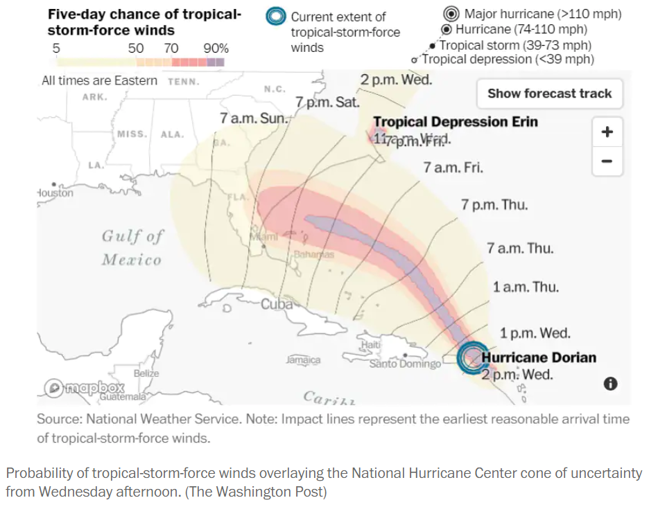
For example, a probabilistic model of a particular Atlantic Hurricane does not provide a mathematical formula for computing the probability that the hurricane makes landfall in the U.S. Nor does the model provide a comprehensive list of the uncountably many possible paths of the hurricane. Rather, the model reflects a set of assumptions under which possible paths can be simulated to approximate probabilities of events of interest like those depicted in Figure 3.1.

Figure 3.1: Picture of a “hurricane cone of uncertainty” from the August 28, 2019 *Washington Post* article “How the hurricane cone of uncertainty can be a cone of confusion, and what to do about it.”

In this chapter we will use simulation to investigate some of the problems introduced in the previous chapter. We can solve many of these problems without simulation. But we like to introduce simulation via simple examples where we know the answers so we can get comfortable with the simulation process and easily check that it works.

3.1 Tactile simulation: Boxes and spinners

While we generally use technology to conduct large scale simulations, it is helpful to first consider how to conduct a simulation by hand using physical objects like coins, dice, cards, or spinners.

Many random phenomena can be represented in terms of a “box model²”

Imagine a box containing “tickets” with labels. Examples include:
- Fair coin flip. 2 tickets: 1 labeled H and 1 labeled T
- Free throw attempt of a 90% free throw shooter. 10 tickets: 9 labeled “make” and 1 labeled “miss”
- Card shuffling. 52 cards: each card with a pair of labels (face value, suit).
The tickets are shuffled in the box and some number are drawn out, either with replacement or without replacement of the tickets before the next draw³.
In some cases, the order in which the tickets are drawn matters; in other cases the order is irrelevant. For example,
- Dealing a 5 card poker hand: Select 5 cards without replacement, order does not matter
- Random digit dialing: Select 4 cards with replacement from a box with tickets labeled 0 through 9 to represent the last 4 digits of a randomly selected phone number with a particular area code and exchange; order matters, e.g., 805-555-1212 is a different outcome than 805-555-2121.
Then something is done with the tickets to determine which events of interest have occurred or to measure random variables. For example, you might flip a coin 10 times (by drawing from the H/T box 10 times with replacement) and check if there were at least 3 H in a row or count the number of H.

If the draws are made with replacement from a single box, we can think of a single circular “spinner” instead of a box, spun multiple times. For example:

Fair coin flip. Spinner with half of the area corresponding to H and half T
Free throw attempt of a 90% free throw shooter. Spinner with 90% of the area corresponding to “make” and 10% “miss”.

Example 3.1 Consider a box model for rolling a four-sided die.

Set up a box model for simulating a roll of each of the following dice.
1. a fair four-sided die
2. the weighted die in Example 2.29
3. the weighted die in Example 2.30.
Roll a die from the previous part twice and let $X$ be the sum of two rolls and let $Y$ be the larger of the two rolls (or the common value if a tie). Explain how you would use the box models from the previous part to simulate a realization of $(X, Y)$.
Let $A$ be the event that the sum is 3, and let $\textrm{I}_A$ be the indicator random variable. Explain how you would use the box models to simulate a realization of $A$ and $I_A$.
In the previous parts, could you use spinners instead?
Use a fair four-sided die (or a box or a spinner) to simulate 10 repetitions. (Yes, really do it.) For each repetition, record the results of the first and second rolls (or draws or spins) and the simulated values of $X$, $Y$, $A$, and $I_A$.

Solution (click to expand)

Solution 3.1.

Each box would have the numbers 1, 2, 3, 4 written on some number of tickets.
1. 4 tickets: labeled 1, 2, 3, 4
2. 10 tickets: 1 labeled 1, 2 labeled 2, 3 labeled 3, 4 labeled 4
3. 15 tickets: 4 labeled 1, 6 labeled 2, 3 labeled 3, 2 labeled 4
Use the appropriate box for the die of interest. Draw two tickets with replacement (that is, put the first ticket back in the box and reshuffle before drawing the second ticket). Let $X$ be the sum of the two numbers drawn and $Y$ the larger of the two numbers drawn.
Similar to the previous part, but event $A$ either happens or not, so a realization of it is true or false instead of a number. If the first roll is 3 then $A$ is true; otherwise $A$ is false. The indicator random variable $\textrm{I}_A$ just translates true to 1 and false to 0.
We could replace the boxes in part 1 with the spinners in Figure 2.9. Spin the appropriate spinner twice and let $X$ be the sum of the two numbers spun and $Y$ the larger of the two numbers spun, etc.
See Table 3.1. Results vary naturally so your simulation results will be different, but the same ideas apply.

Table 3.1: Results of 10 repetitions of two rolls of a fair four-sided die. X is the sum of the two rolls, Y is the maximum, and A is the event that the first roll is a 3.

Repetition	First roll	Second roll	X	Y	Event A occurs?	I[A]
1	2	1	3	2	False	0
2	1	1	2	1	False	0
3	3	3	6	3	True	1
4	4	3	7	4	False	0
5	3	2	5	3	True	1
6	3	4	7	4	True	1
7	2	3	5	3	False	0
8	2	4	6	4	False	0
9	1	2	3	2	False	0
10	3	4	7	4	True	1

Warning

The tables of outcomes in this chapter are a different type than those in Chapter 2. Many tables in Chapter 2, such as Table 2.7, represent the sample space: there is one and only one row for each distinct possible outcome, and each outcome (row) has a corresponding theoretical probability. On the other hand, tables of simulation output—like Table 3.1 and many tables in this chapter—contain one row for each repetition of the simulation. A particular outcome might be repeated several times in a simulation and thus might appear in several rows of the table of simulation output. For example, the outcome (3, 4) appears only once in Table 2.7, but twice in Table 3.1 (in repetitions 6 and 10). We will discuss how to approximate the theoretical probability of a particular outcome using the relative frequency of repetitions of that outcome in the simulation.

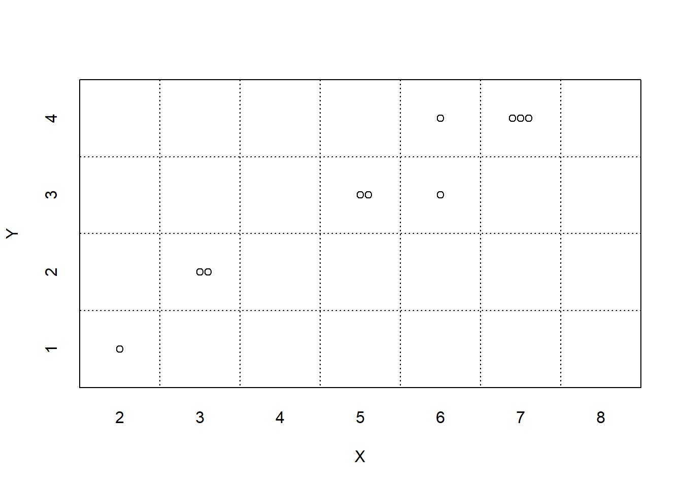
Note that we are able to simulate outcomes of the rolls and values of $X$ and $Y$ without defining the probability space in detail. That is, we do not need to list all the possible outcomes and events and their probabilities. Instead, the probability space is defined implicitly via the specification to “roll a fair four-sided die twice” or “draw two tickets with replacement from a box with four tickets labeled 1, 2, 3, 4” or “spin the spinner on the left of Figure 2.9 twice”. The random variables are defined by what is being measured for each outcome, the sum ($X$) and the max ($Y$) of the two draws or spins.

A simulation usually involves many repetitions. When conducting a simulation⁴ it is important to distinguish between what entails (1) one repetition of the simulation and its output, and (2) the simulation itself and output from many repetitions. When describing a simulation, refrain from making vague statements like “repeat this” or “do it again”, because “this” or “it” could refer to different elements of the simulation. In the dice example, (1) rolling a die is repeated to generate a single $(X, Y)$ pair, and (2) the process of generating $(X, Y)$ pairs is repeated to obtain the simulation results. That is, a single repetition involves an ordered pair of die rolls, resulting in an outcome $\omega$, and the values of the sum $X(\omega)$ and max $Y(\omega)$ are computed for the outcome $\omega$. The process described in the previous sentence is repeated many times to generate many outcomes and $(X, Y)$ pairs according to the probability model.

Think of simulation results being organized in a table like Table 3.1, where each row corresponds to a repetition of the simulation, resulting in a possible outcome of the random phenomenon, and each column corresponds to a different random variable or event. Remember that indicators are the bridge between events and random variables. On each repetition of the simulation an event either occurs or not; we could record the occurrence of an event as “true” or “false”, or we could record the value of the corresponding indicator random variable, 1 or 0.

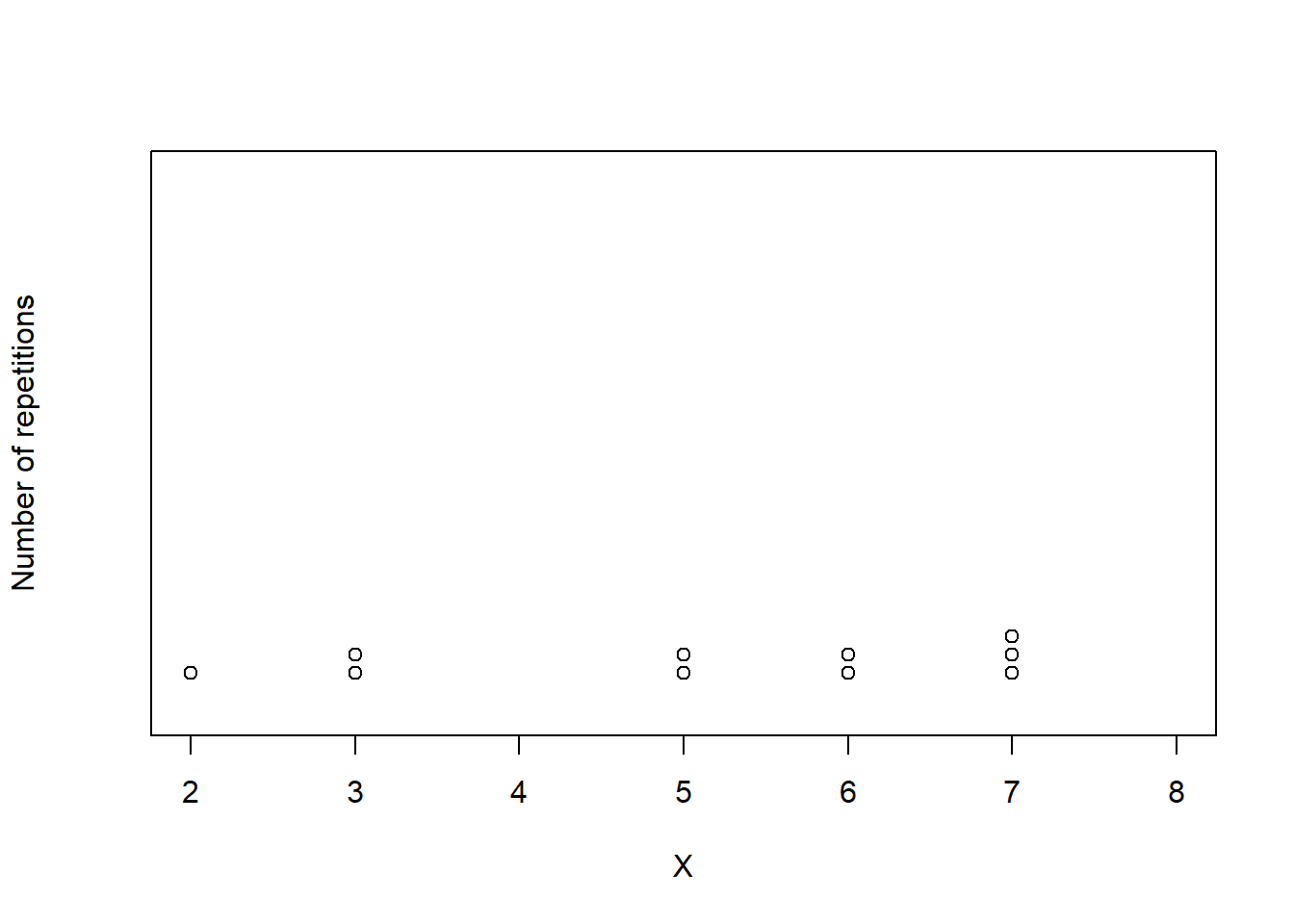
Figure 3.2 displays two plots summarizing the results in Table 3.1. Each dot represents the results of one repetition. Figure 3.2 (a) displays the simulated $(X, Y)$ pairs, Figure 3.2 (b) displays the simulated values of $X$ alon along with their frequencies. While this simulation only consists of 10 repetitions, a larger scale simulation would follow the same process.

Example 3.2 Recall Example 2.2. Consider the matching problem with $n=4$. Label the objects 1, 2, 3, 4, and the spots 1, 2, 3, 4, with spot 1 the correct spot for object 1, etc. Let $X$ be the number of objects that are placed in the correct spot, and let $C$ be the event that at least one object is placed in the correct spot. Describe how you would use a box model to simulate a single realization of $X$ and of $C$. Could you use a spinner instead?

Solution (click to expand)

Solution 3.2. Use a box with 4 tickets, labeled 1, 2, 3, 4. Shuffle the tickets and draw all 4 without replacement and record the tickets drawn in order. Let $X$ be the number of tickets that match their spot in order. For example, if the tickets are drawn in the order 2431 then the realized value of $X$ is 1 since only ticket 3 matches its spot in the order. Since $C=\{X \ge 1\}$, event $C$ occurs if $X\ge 1$ and does not occur if $X=0$. We could record the realization of event $C$ as “true” or “false”. We could also record the realization of $\textrm{I}_C$, the indicator random variable for event $C$, as 1 if $C$ occurs and 0 if $C$ does not occur.

Since the tickets are drawn without replacement, we could not simply spin a single spinner, like the one in Figure 2.9 (a), four times. If we really wanted to use the spinner in Figure 2.9 (a), we couldn’t just spin it four times; we would sometimes have to discard spins and try again. For example, suppose the first spin results in 2; then if the second spin results in 2 we would need to discard it and try again. So we would usually need more than four spins to obtain a valid outcome. If we wanted to guarantee a valid outcome in only four spins, we would need a collection of spinners, and which one we use would depend on the results of previous spins. For example, if the first spin results in 2, then we would need to spin a spinner that only lands on 1, 3, 4; if the second spin results in 3, then we would need to spin a spinner that lands only on 1 and 4.

3.1.1 Exercises

Exercise 3.1 Recall the birthday problem of Example 2.48. Let $B$ be the event that at least two people in a group of $n$ share a birthday.

Describe in detail you could use physical objects (coins, cards, spinners, etc) to simulate by hand a single realization of $B$ (that is, simulate whether or not $B$ occurs).

Exercise 3.2 Maya is a basketball player who makes 40% of her three point field goal attempts. Suppose that at the end of every practice session, she attempts three pointers until she makes one and then stops. Let $X$ be the total number of shots she attempts in a practice session. Assume shot attempts are independent, each with probability of 0.4 of being successful. Describe in detail you could use physical objects (coins, cards, spinners, etc) to simulate by hand a single value of $X$.

Exercise 3.3 The latest series of collectible Lego Minifigures contains 3 different Minifigure prizes (labeled 1, 2, 3). Each package contains a single unknown prize. Suppose we only buy 3 packages and we consider as our sample space outcome the results of just these 3 packages (prize in package 1, prize in package 2, prize in package 3). For example, 323 (or (3, 2, 3)) represents prize 3 in the first package, prize 2 in the second package, prize 3 in the third package. Let $X$ be the number of distinct prizes obtained in these 3 packages. Let $Y$ be the number of these 3 packages that contain prize 1.

Describe in detail you could use physical objects (coins, cards, spinners, etc) to simulate by hand a single $(X, Y)$ pair.

3.2 Tactile simulation: Meeting problem

Now we’ll consider tactile simulation for a continuous sample space. Throughout this section we’ll consider the two-person meeting problem. We’ll continue to measure arrival times in minutes after noon, including fractions of a minute, so that arrival times take values on a continuous scale.

3.2.1 A uniform distribution

Example 3.3 Assume that Regina and Cady each arrive at a time uniformly at random in the continuous time interval between noon and 1, independently of each other.

Explain how you could construct a circular spinner to simulate Regina’s arrival time. In particular, what values go at the “3 o’clock”, “6 o’clock”, and “9 o’clock” points on the spinner’s axis? (Here “3 o’clock” refers to the direction on the “clock” (spinner), and not arrival time.)
Explain how you could use the spinner from the previous part to simulate an outcome, that is, a pair of arrival times for Regina and Cady.
Why could we not simulate this situation with a box model?

Solution (click to expand)

Solution 3.3.

Imagine a circular spinner with an infinitely fine needle that after being spun well points to a value on the spinner’s axis uniformly at random. We could label the axis like the spinner like the one in Figure 2.1, but ranging from 0 to 60 instead of 0 to 1; see Figure 3.3, which we’ll call the “Uniform(0, 60)” spinner. (Or we could just use the spinner in Figure 2.1 to get the arrival time as a fraction of the hour, then multiply the result of a spin by 60.) Only selected rounded values are displayed on the circular axis, but in the idealized model the spinner is infinitely precise so that any real number between 0 and 60 is a possible outcome. Assuming the arrival time is uniformly distributed, Regina should have a probability of $15/60=0.25$ of arriving in each of the 15-minutes intervals $[0, 15]$, $[15, 30]$, $[30, 45]$, and $[45, 60]$. Therefore, 15 should go at “3 o’clock”, 30 at “6 o’clock”, and 45 at “9 o’clock”, just like the minutes on a regular clock.
Since the arrival times are independent and follow the same uniform pattern, we can spin the spinner in Figure 3.3 twice to simulate an outcome; the first spin represents Regina’s arrival time, the second Cady’s. The order of the spins matters; for example, the pair (34.89, 12.56) represents Regina arriving at 34.89 minutes after noon, while the pair (12.56, 34.89) represents Regina arriving at 12.56 minutes after noon (and vice versa for Cady).
An outcome consists of a pair of values from the continuous interval [0, 60]. Since this interval is uncountable, it’s not possible to write every real number in the interval [0, 60] on a ticket to place in a box. To use a box model, we would have to round arrival times to some desired degree of precision—nearest minute, second, millisecond, etc—and put the rounded values on the tickets. Which is probably fine for practical purposes! But if we really want to create a tactile representation of continuous outcomes, a box model won’t work; we tend to use spinners instead.

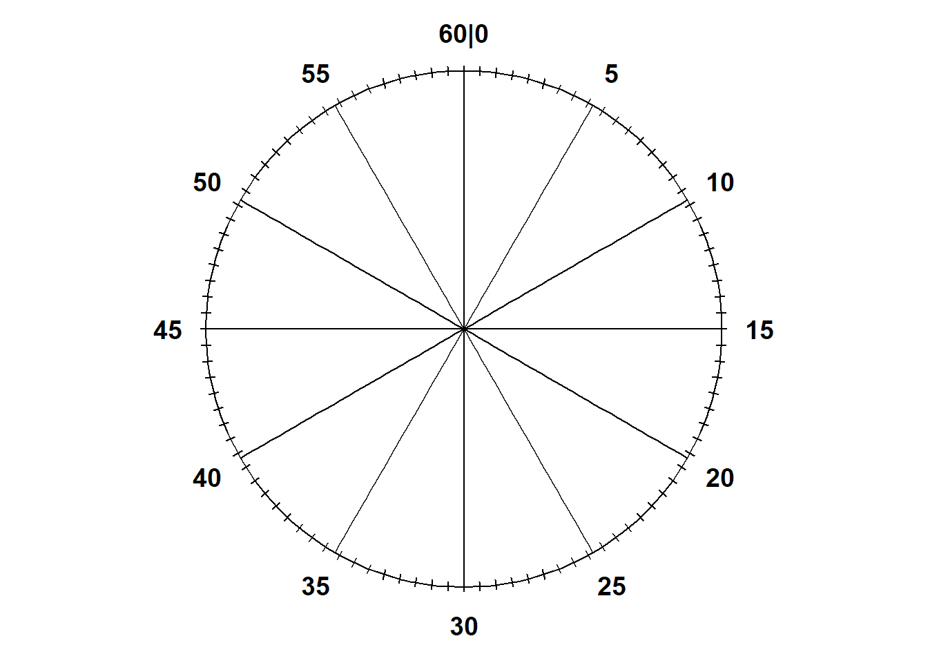
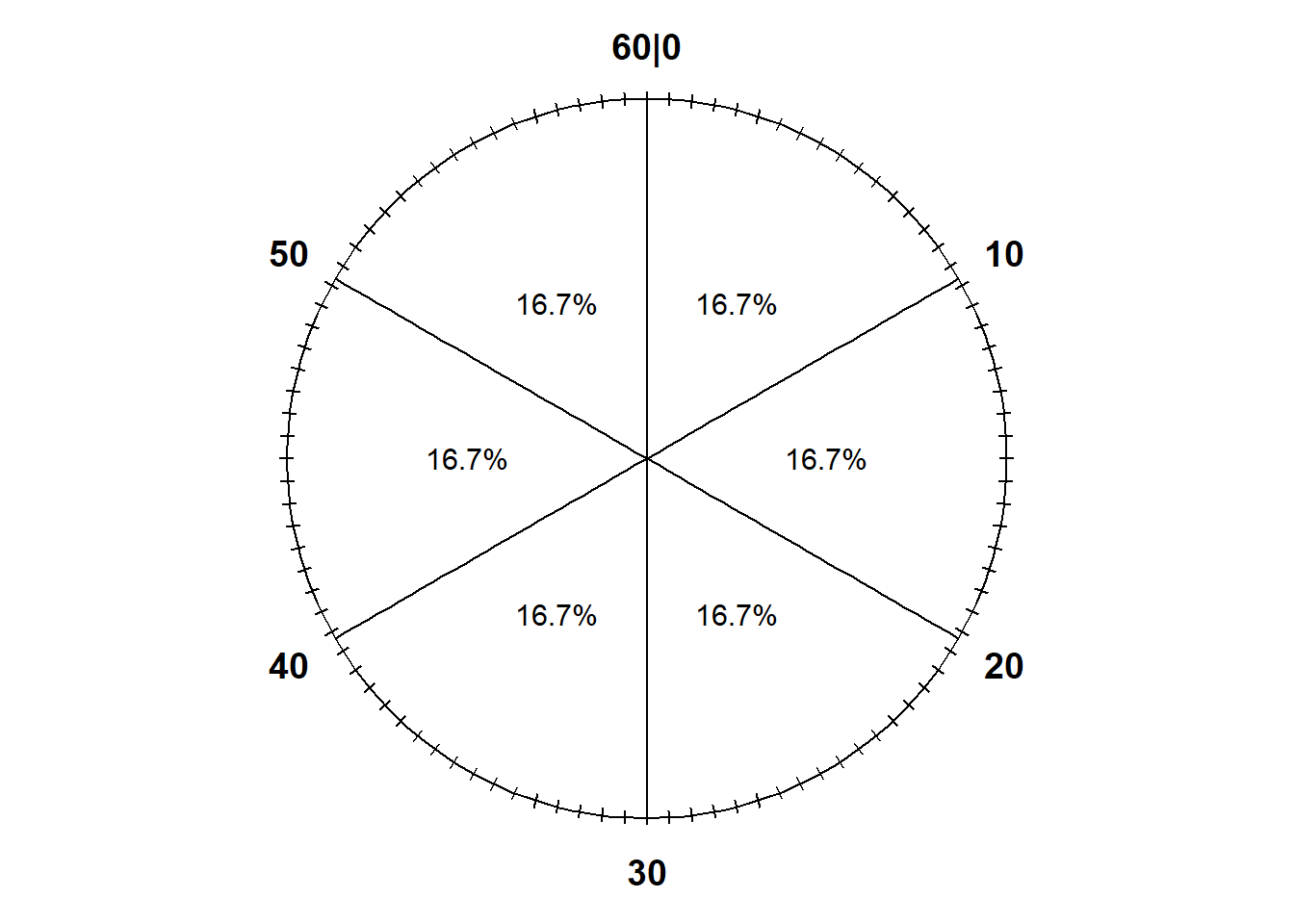
Notice that the values on the circular axis in Figure 3.3 are evenly spaced. For example, the intervals [0, 15], [15, 30], [30, 45], and [45, 60], all of length 15, each represent 25% of the spinner area. If we spin the idealized spinner represented by Figure 3.3 10 times, our results might look like those in Table 3.2.

Table 3.2: Results of 10 spins of the Uniform(0, 60) spinner.

Results of 10 spins of the Uniform(0, 60) spinner.
Spin	Result
1	1.062914
2	17.729239
3	21.610468
4	27.190663
5	36.913450
6	19.604730
7	14.479123
8	25.198875
9	2.805937
10	17.456726

Notice the number of decimal places. If the sample space is [0, 60], any value in the continuous interval between 0 and 60 is a distinct possible value: 10.25000000000… is different from 10.25000000001… which is different from 10.2500000000000000000001… and so on.

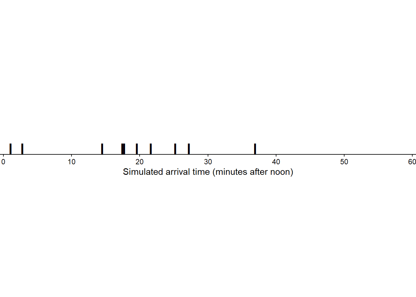
Figure 3.4 displays the 10 values in Table 3.2 plotted along a number line. The values are roughly evenly spaced, but there is some natural variability. (Though it’s hard to discern any pattern with only 10 values.)

Figure 3.4: Plot of the 10 values simulated from a Uniform(0, 60) model, recorded in Table 3.2

To simulate a (Regina, Cady) pair of arrival times, we would spin the Uniform(0, 60) spinner twice. Let $R$ be the result of the first spin, representing Regina’s arrival time, and $Y$ the second spin for Cady. Also let $T=\min(R, Y)$ be the time (minutes after noon) at which the first person arrives, and $W=|R-Y|$ be the time (minutes) the first person to arrive waits for the second person to arrive. Table 3.3 displays the values of $R$, $Y$, $T$, $W$ for 10 simulated repetitions, each repetition consisting of a pair of spins of the Uniform(0, 60) spinner.

Table 3.3: Results of 10 repetitions of a simulation of the independent Uniform model in the two-person meeting problem.

Results of 10 repetitions of a simulation of the independent Uniform model in the two-person meeting problem.
Repetition	R	Y	T	W
1	49.50512	52.748971	49.505123	3.243848
2	55.38527	22.040907	22.040907	33.344360
3	7.52414	9.956804	7.524140	2.432664
4	51.33105	39.636179	39.636179	11.694869
5	43.77325	26.338476	26.338476	17.434775
6	42.51350	28.619413	28.619413	13.894083
7	31.15456	41.117529	31.154557	9.962971
8	44.01602	4.406319	4.406319	39.609700
9	35.46720	8.867082	8.867082	26.600122
10	56.58527	7.784337	7.784337	48.800934

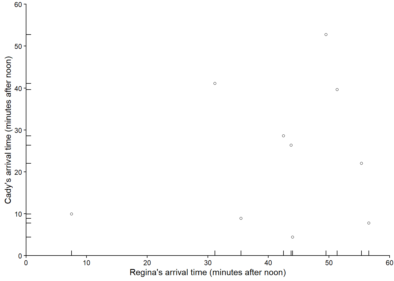
Figure 3.5 plots the 10 simulated $(R, Y)$ pairs in Table 3.3

Figure 3.5: Plot of 10 pairs of values, each pair simulated independently from a Uniform(0, 60) model, recorded in Table 3.3. Each dot represents a pair. The components of each pair are marked on the horizontal and vertical axes.

Now suppose we keep repeating the process, resulting in many simulated (Regina, Cady) pairs of arrival times. Figure 3.6 displays 1000 simulated pairs of arrival times, resulting from 1000 pairs of spins of the Uniform(0, 60) spinner.

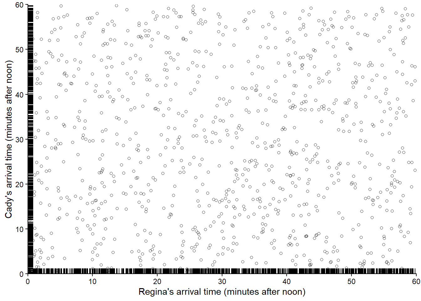
Figure 3.6: Plot of 1000 pairs of values, each pair simulated independently from a Uniform(0, 60) model. Each dot represents a pair. The components of each pair are marked on the horizontal and vertical axes.

We see that the pairs are fairly evenly distributed throughout the square with sides [0, 60] representing the sample space (though there is some “clumping” due to natural variability). If we simulated more values and summarized them in an appropriate plot, we would expect to see something like Figure 2.12.

3.2.2 A non-uniform distribution

Example 3.4 Imagine we have an unlabeled circular spinner with an infinitely fine needle that after being spun well lands on a point on the spinner’s axis uniformly at random. But now suppose that Regina’s arrival time is not uniformly distributed. How should we label the spinner’s circular axis to reflect assumptions about Regina’s arrival time?

In particular, suppose that Regina has a probability of 0.25 of arriving in each of the intervals $[0, 23]$, $[23, 30]$, $[30, 37]$, $[37, 60]$. Start to label the spinner for simulating Regina’s arrival time; what values should go at the “3 o’clock”, “6 o’clock”, and “9 o’clock” positions on the spinner’s circular axis?
Also assume that Regina has a probability of (roughly):
- 0.025 of arriving in the interval $[0, 10]$
- 0.135 of arriving in the interval $[10, 20]$
- 0.135 of arriving in the interval $[40, 50]$
- 0.025 of arriving in the interval $[50, 60]$
At what points on the spinner’s circular axis should the values 10, 20, 40, and 50 go? What is the probability that Regina arrives in the interval $[20, 30]$? $[30, 40]$?
What does this spinner say about Regina’s arrival time: is she most likely to arrive near noon, near 12:30, or near 1:00?

Solution (click to expand)

Solution 3.4.

We can split the spinner into four equal sectors representing the four intervals. Therefore, 23 should go at 3 o’clock, 30 at 6 o’clock, and 37 at 9 o’clock. See Figure 3.7 (a). This part only provides enough information to label 3, 6, and 9 o’clock; we’ll discuss where the other values come from below. (Also, we have rounded values in this example.)
Starting from 0 and moving clockwise around the spinner
- 10 goes 2.5% of the way around
- 20 goes 16% of the way around, at roughly 2 o’clock (2.5% to get from 0 to 10 then another 13.5% to get from 10 to 20)
- 30 goes at 6 o’clock like before
- 40 goes 84% of the way around, at roughly 10 o’clock ($1 - 0.025 - 0.135 = 0.84$)
- 50 goes 97.5% of the way around ($1 - 0.025 = 0.975$) Since the probability of arriving in $[0, 30]$ is 0.5, the probability of arriving in $[20, 30]$ is $0.5 - 0.16 = 0.34$. Similarly, the probability of arriving in $[30, 40]$ is 0.34. See Figure 3.7 (b) (We have rounded values a little differently for this example.)
Part 1 shows that Regina is as likely as not to arrive between 12:23 and 12:37. Part 2 shows that Regina has a probability of about 0.68 of arriving withing 10 minutes of 12:30, but only a probability of about 0.05 of arriving within 10 minutes of either noon or 1:00. So under these assumptions she is more likely to arrive near 12:30 than near noon or 1:00.

Imagine we have an unlabeled circular spinner with an infinitely fine needle that after being spun well lands on a point on the spinner’s axis uniformly at random. Even though the needle lands uniformly, we can use the spinner to represent non-uniform probability measures by labeling the spinner’s circular axis appropriately. We can “stretch” intervals with higher probability, and “shrink” intervals with lower probability. We have already done this intuitively with discrete spinners; see Figure 1.6 and Figure 2.9. But the same idea applies to continuous spinners.

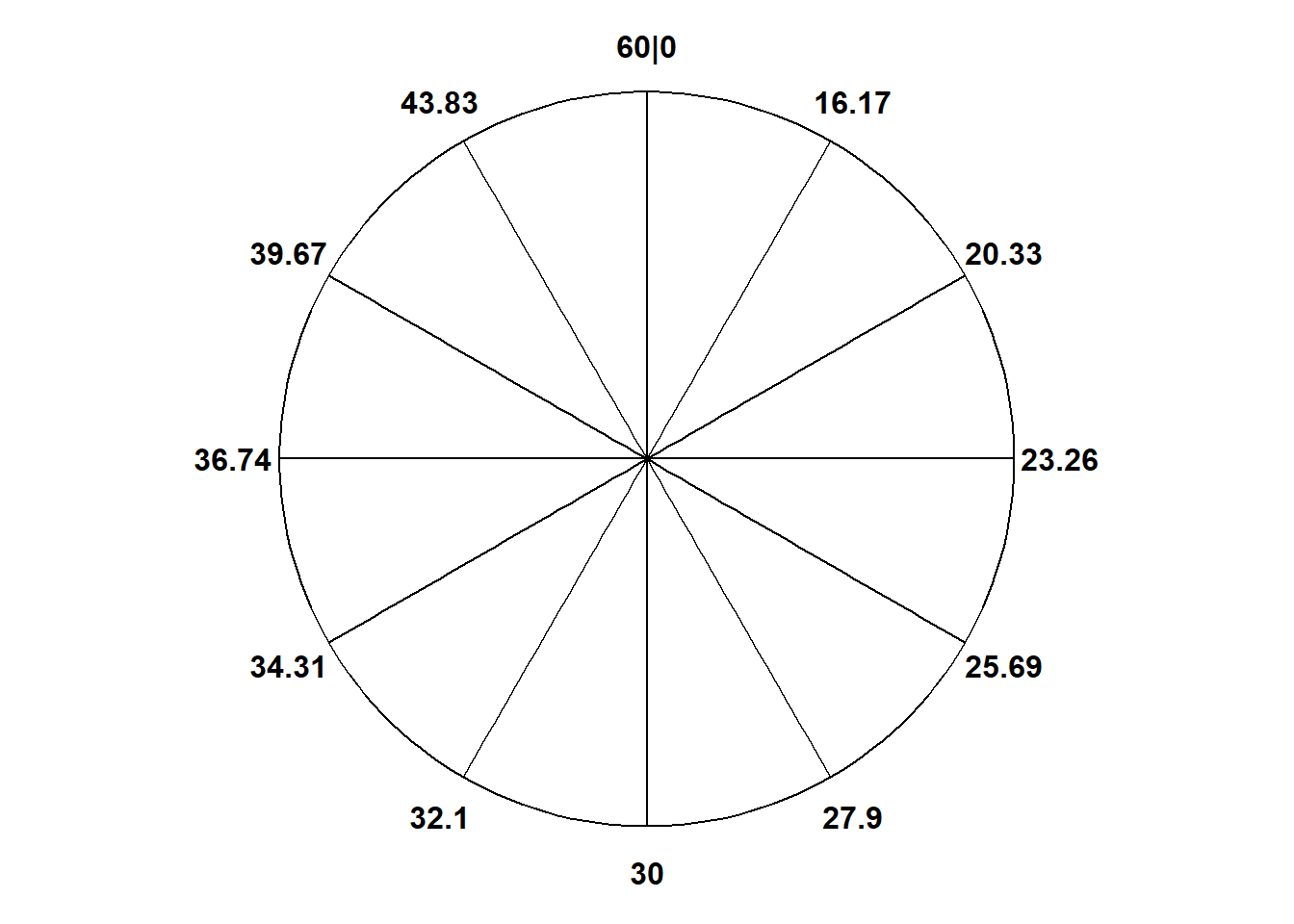
Figure 3.7 displays a “Normal(30, 10)” spinner. Only selected rounded values are displayed, but the needle can land—uniformly at random—at any point on the continuous circular axis. But pay close attention to the circular axis; the values are not equally spaced. For example, the bottom half of the spinner corresponds to the interval [23.26, 36.74], with length 13.48 minutes, while the upper half of the spinner corresponds to the intervals [0, 23.26] and [36.74, 60], with total length 46.52 minutes. Compared with the Uniform(0, 60) spinner, in the Normal(30, 10) spinner intervals near 30 are “stretched out” to reflect a higher probability of arriving near 12:30, while intervals near 0 and 60 are “shrunk” to reflect a lower probability of arriving near 12:00 or 1:00. The interval [20, 40] represents about 68% of the spinner area, so if we spin this spinner many times, about 68% of the spins will land in the interval [20, 40]. A person whose arrival time is represented by this spinner has a probability of about 0.68 of arriving within 10 minutes of 12:30 compared to $20/60 = 0.33$ for the Uniform(0, 60) model, and a probability of about 0.05 of arriving with 10 minutes of either noon or 1:00, compared to $20/60=0.33$ in the Uniform(0, 60) model. (The spinner on the left is divided into 12 wedges of equal area, so each wedge represents 8.33% of the probability. Not all values on the axis are labeled, but you can use the wedges to eyeball probabilities.)

The particular pattern represented by the spinner in Figure 3.7 is a Normal(30, 10) distribution; that is, a Normal distribution with mean 30 and standard deviation 10. We will see Normal distributions in much more detail later. For now, just know that a Normal(30, 10) model reflects one particular pattern of non-uniform probability⁵. Table 3.4 compares probabilities of selected intervals under the Uniform(0, 60) and Normal(30, 10) models.

Warning

The parameters in the uniform probability model are different from those in the Normal model. In the Uniform(0, 60) model, 0 is the minimum possible value; in the Normal(30, 10) model, 30 is the average value. In the Uniform(0, 60) model, 60 is the maximum possible value; in the Normal(30, 10) model, 10 is the standard deviation.

Table 3.4: Comparison of probabilities for the Uniform(0, 60) and Normal(30, 10) models

Interval	Uniform(0, 60) probability	Normal(30, 10) probability
[0, 10]	0.167	0.025
[10, 20]	0.167	0.136
[20, 30]	0.167	0.341
[30, 40]	0.167	0.341
[40, 50]	0.167	0.136
[50, 60]	0.167	0.025

If we spin the idealized spinner represented by Figure 3.7 10 times, our results might look like those in Table 3.5.

Table 3.5: Results of 10 spins of the Normal(30, 10) spinner.

Spin	Result
1	21.38732
2	50.71937
3	24.08964
4	32.68036
5	54.51060
6	38.11696
7	16.81857
8	22.97995
9	28.86703
10	43.43031

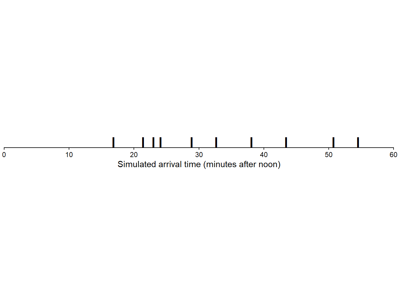
Figure 3.8 displays the 10 values in Table 3.5 plotted along a number line. We tend to see more values near 30 than near 0 or 60 (though it’s hard to discern any pattern with only 10 values).

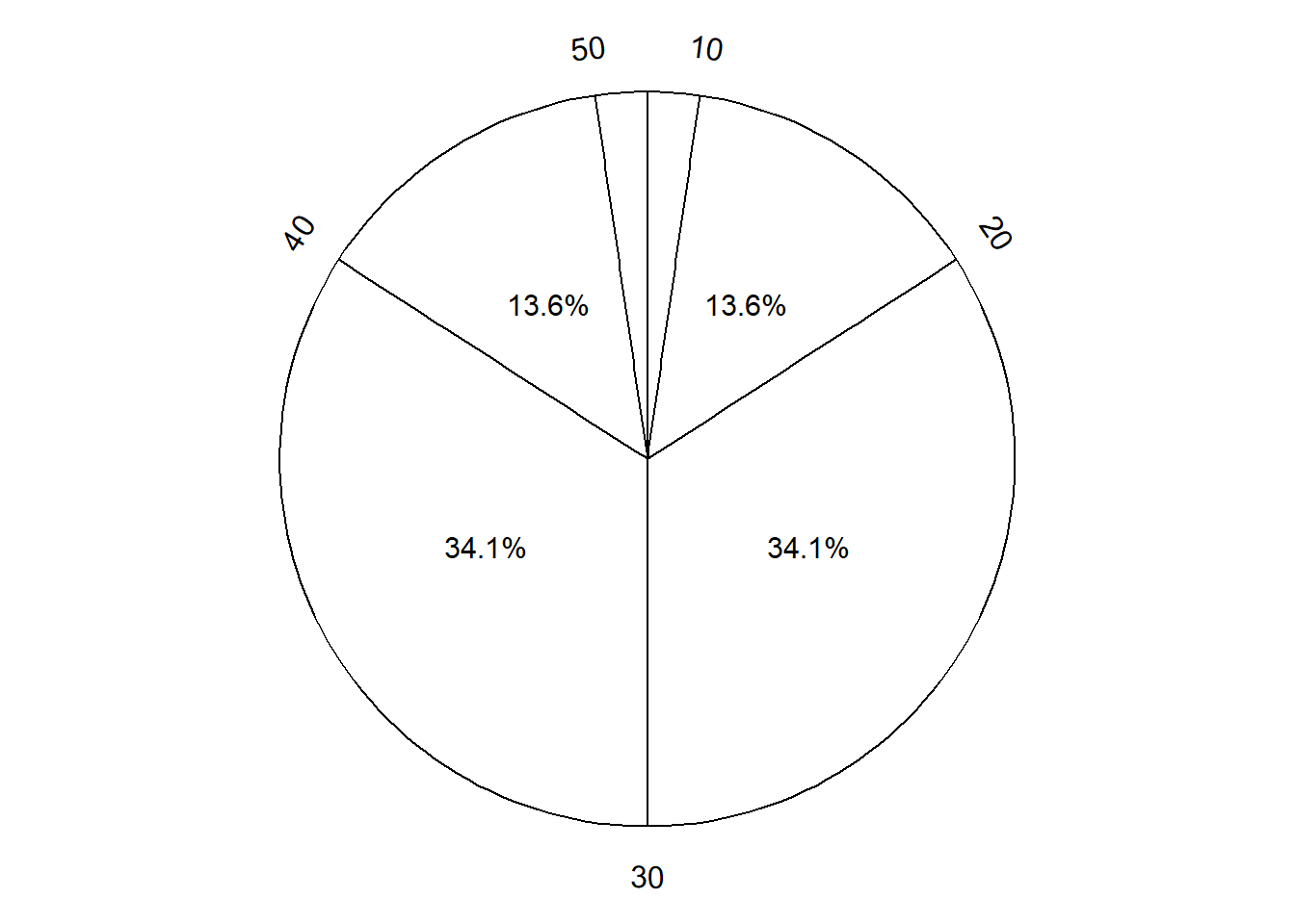
Figure 3.8: Plot of the 10 values simulated from a Normal(30, 10) model, recorded in Table 3.5.

If we spin the spinner in Figure 3.7 many times,

About half of the simulated values would be below 30 and half above
Because axis values near 30 are stretched out, values near 30 would occur with higher frequency than those near 0 or 60.
The shape of the distribution would be symmetric about 30 since the axis spacing of values below 30 mirrors that for values above 30. For example, about 34% of values would be between 20 and 30, and also 34% between 30 and 40.
About 68% of values would be between 20 and 40.
About 95% of values would be between 10 and 50.

And so on. We could compute percentages for other intervals by measuring the areas of corresponding sectors on the spinner to complete the pattern of variability that values resulting from this spinner would follow. This particular pattern is called a “Normal(30, 10)” distribution, which we will explore in much more detail later (in particular, see Section 5.3).

Now suppose Regina’s and Cady’s arrival times are each reasonably modeled by a Normal(30, 10) model, independently of each other. To simulate a (Regina, Cady) pair of arrival times, we would spin the Normal(30, 10) spinner twice. Table 3.6 displays the results of 10 repetitions, each repetition resulting in a (Regina, Cady) pair.

Table 3.6: Results of 10 pairs of spins of the Normal(30, 10) spinner.

Repetition	Regina's time	Cady's time
1	31.758630	50.89160
2	7.842356	34.23954
3	29.644008	40.34209
4	25.154312	26.89845
5	38.011497	32.04975
6	27.325808	42.97185
7	44.594399	38.65448
8	18.557759	30.99171
9	30.142711	36.53947
10	26.479249	30.23044

Figure 3.9 plots the 10 simulated pairs in Table 3.6

Figure 3.9: Plot of 10 pairs of values, each pair simulated from a Normal(30, 10) model, recorded in Table 3.6. Each dot represents a pair. The components of each pair are marked on the horizontal and vertical axes.

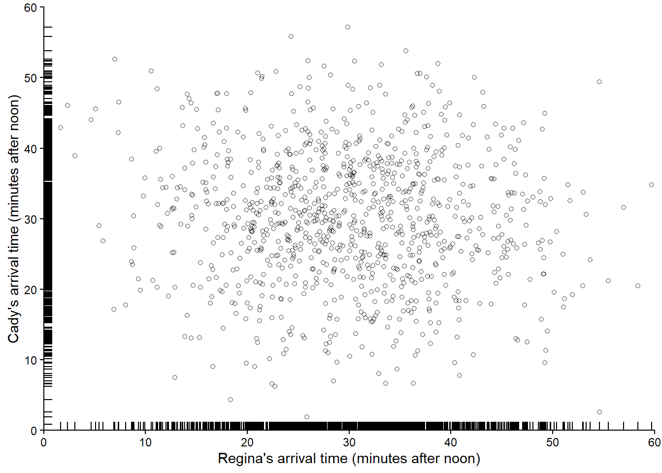
Figure 3.10 displays 1000 pairs of (Regina, Cady) arrival times, resulting from 1000 pairs of spins of the Normal(30, 10) spinner. Compared with the simulated pairs from the Uniform(0, 60) spinner (in Figure 3.6), we see many more simulated pairs in the center of the plot (when both arrive near 12:30) than in the corners of the plot (where either arrives near 12:00 or 1:00). If we simulated more values and summarized them in an appropriate plot, we would expect to see something like Figure 2.14.

Figure 3.10: Plot of 1000 pairs of values, each pair simulated from a Normal(30, 10) model. Each dot represents a pair. The components of each pair are marked on the horizontal and vertical axes.

Example 3.3 and Example 3.4 assumed that Regina’s and Cady’s arrival times individually followed the same model, both Uniform(0, 60) or both Normal(30, 10), so we just spun the same spinner twice to simulate a pair of arrival times. However, we could easily simulate from different models. Suppose Regina’s arrival time follows a Uniform(0, 60) model while Cady’s follows a Normal(30, 10) model, independently of each other. Then we could simulate a pair of arrival times by spinning the Uniform(0, 60) spinner for Regina and the Normal(30, 10) spinner for Cady.

So far we have assumed that Regina and Cady arrive independently, but what if they coordinate and their arrival times are related? Recall that Figure 2.15 reflects a model where Regina and Cady each are more likely to arrive around 12:30 than noon or 1:00, and also more likely to arrive around the same time. In such a situation, we could still use spinners to simulate pairs of arrival times, but it’s more involved than just spinning a single spinner twice (or having just one spinner for each person). We’ll revisit using spinners to simulate dependent pairs later.

3.2.3 Exercises

Exercise 3.4 Katniss throws a dart at a circular dartboard with radius 12 inches. Suppose that the dart lands uniformly at random anywhere on the dartboard, and assume that Katniss’s dart never misses the dartboard. Suppose that the dartboard is on a coordinate plane, with the center of the dartboard at (0, 0) and the north, south, east, and west edges, respectively, at coordinates (0, 12), (0,-12), (12, 0), (-12, 0). When the dart hits the board its $(X, Y)$ coordinates are recorded. Let $R$ be the distance (inches) from the location of the dart to the center of the dartboard.

Sketch a Uniform(0, 12) spinner.
Describe how you could use a fair coin and the Uniform(0, 12) spinner to simulate the $(X, Y)$ coordinates of a single throw of the dart and the value of $R$. Hint: you might need to flip the coin and spin the spinner multiple times. What will you do if your simulated coordinates correspond to “off the board”?
Suppose you want to simulate $R$ directly. Could you just spin the Uniform(0, 12) spinner and record the value? Explain. Hint: see Exercise 2.13.

Exercise 3.5 Continuing Exercise 3.4. Computing like we did in Exercise 2.13, we can show

Range	Probability that $R$ is in range
0 to 1	0.0069
1 to 2	0.0208
2 to 3	0.0347
3 to 4	0.0486
4 to 5	0.0625
5 to 6	0.0764
6 to 7	0.0903
7 to 8	0.1042
8 to 9	0.1181
9 to 10	0.1319
10 to 11	0.1458
11 to 12	0.1597

Sketch a spinner that could be used to simulate values of $R$. You should label 12 sectors on the spinner. Hint: the sectors won’t be the same size and the values on the outside axis of the spinner won’t be evenly spaced.

3.3 Computer simulation: Dice rolling

We will perform computer simulations using the Python package Symbulate. The syntax of Symbulate mirrors the language of probability in that the primary objects in Symbulate are the same as the primary components of a probability model: probability spaces, random variables, events. Once these components are specified, Symbulate allows users to simulate many times from the probability model and summarize the results.

This section contains a brief introduction to Symbulate; more examples can be found throughout the text. Symbulate can be installed with pip.

pip install git+https://github.com/kevindavisross/symbulate

Import Symbulate during a Python session using the following command.

from symbulate import *

We’ll start with a dice rolling example. Unless indicated otherwise, in this section $X$ represents the sum of two rolls of a fair four-sided die, and $Y$ represents the larger of the two rolls (or the common value if a tie). We have already discussed a tactile simulation; now we’ll carry out the process on a computer.

There aren’t many examples for you to work in this section. Instead, we encourage you to open a Python session and copy and run the code as you read. In particular, you can run Python code using this template Colab notebook which includes the code needed to get started with Symbulate.

3.3.1 Simulating outcomes

The following Symbulate code defines a probability space⁶ P for simulating the 16 equally likely ordered pairs of rolls via a box model.

P = BoxModel([1, 2, 3, 4], size = 2, replace = True)

The above code tells Symbulate to draw 2 tickets (size = 2), with replacement⁷, from a box with tickets labeled 1, 2, 3, and 4 (entered as the Python list [1, 2, 3, 4]). Each simulated outcome consists of an ordered⁸ pair of rolls .

The sim(r) command simulates r realizations of probability space outcomes (or events or random variables). Here is the result of one repetition.

P.sim(1)

Index	Result
0	(4, 4)

And here are the results of 10 repetitions. (We will typically run thousands of repetitions, or more, but in this section we just run a few repetitions for illustration.)

P.sim(10)

Index	Result
0	(1, 3)
1	(1, 3)
2	(2, 4)
3	(1, 2)
4	(1, 2)
5	(1, 4)
6	(3, 1)
7	(2, 3)
8	(2, 3)
...	...
9	(3, 2)

Warning

Every time .sim() is called, a new simulation is run. When running a simulation, the “simulate” step should be performed with a single call to sim so that all analysis of results corresponds to the same simulated values. We’ll show how to do this below.

3.3.2 Simulating random variables

A Symbulate RV is specified by the probability space on which it is defined and the mapping function which defines it. Recall that $X$ is the sum of the two dice rolls and $Y$ is the larger (max).

X = RV(P, sum)
Y = RV(P, max)

The above code simply defines the random variables. Again, we can simulate values with .sim(). Since every call to sim runs a new simulation, we typically store the simulation results as an object. The following commands simulate 100 values of the random variable X and store the results as x. For consistency with standard probability notation⁹, the random variable itself is denoted with an uppercase letter X, while the realized values of it are denoted with a lowercase letter x.

x = X.sim(100)

x # this just displays x; only the first few and last values will print

Index	Result
0	6
1	7
2	4
3	4
4	8
5	5
6	5
7	3
8	6
...	...
99	4

3.3.3 Simulating multiple random variables

If we call X.sim(10000) and Y.sim(10000) we get two separate simulations of 10000 pairs of rolls, one which returns the sum of the rolls for each repetition, and the other the max. If we want to study relationships between $X$ and $Y$ we need to compute both $X$ and $Y$ for each pair of rolls in the same simulation.

We can simulate $(X, Y)$ pairs using¹⁰ &. We store the simulation output as x_and_y to emphasize that x_and_y contains pairs of values.

x_and_y = (X & Y).sim(10)

x_and_y # this just displays x_and_y

Index	Result
0	(4, 3)
1	(5, 4)
2	(3, 2)
3	(3, 2)
4	(5, 3)
5	(6, 3)
6	(5, 4)
7	(7, 4)
8	(4, 3)
...	...
9	(5, 4)

Think of x_and_y as a table with two columns. We can select columns using brackets []. Remember that Python uses zero-based indexing, so 0 corresponds to the first column, 1 to the second, etc.

x = x_and_y[0]

x

Index	Result
0	4
1	5
2	3
3	3
4	5
5	6
6	5
7	7
8	4
...	...
9	5

y = x_and_y[1]

y

Index	Result
0	3
1	4
2	2
3	2
4	3
5	3
6	4
7	4
8	3
...	...
9	4

We can also select multiple columns.

x_and_y[0, 1]

Index	Result
0	(4, 3)
1	(5, 4)
2	(3, 2)
3	(3, 2)
4	(5, 3)
5	(6, 3)
6	(5, 4)
7	(7, 4)
8	(4, 3)
...	...
9	(5, 4)

3.3.4 Simulating outcomes and random variables

When calling X.sim(10) or (X & Y).sim(10) the outcomes of the rolls are generated in the background but not saved. We can create a RV which returns the outcomes of the probability space¹¹. The default mapping function for RV is the identity function, $g(u) = u$, so simulating values of U = RV(P) below returns the outcomes of the BoxModel P representing the outcome of the two rolls.

U = RV(P)

U.sim(10)

Index	Result
0	(1, 4)
1	(3, 3)
2	(4, 3)
3	(3, 1)
4	(4, 3)
5	(1, 2)
6	(3, 4)
7	(3, 1)
8	(3, 3)
...	...
9	(4, 4)

Now we can simulate and display the outcomes along with the values of $X$ and $Y$ using &.

(U & X & Y).sim(10)

Index	Result
0	((4, 4), 8, 4)
1	((1, 2), 3, 2)
2	((1, 1), 2, 1)
3	((2, 1), 3, 2)
4	((3, 3), 6, 3)
5	((2, 3), 5, 3)
6	((4, 4), 8, 4)
7	((2, 4), 6, 4)
8	((3, 4), 7, 4)
...	...
9	((3, 1), 4, 3)

Because the probability space P returns pairs of values, U = RV(P) above defines a random vector. The individual components¹² of U can be “unpacked” as U1, U2 in the following. Here U1 is an RV representing the result of the first roll and U2 the second.

U1, U2 = RV(P)
(U1 & U2 & X & Y).sim(10)

Index	Result
0	(1, 4, 5, 4)
1	(2, 4, 6, 4)
2	(3, 4, 7, 4)
3	(1, 3, 4, 3)
4	(3, 3, 6, 3)
5	(3, 4, 7, 4)
6	(3, 3, 6, 3)
7	(3, 1, 4, 3)
8	(3, 2, 5, 3)
...	...
9	(4, 1, 5, 4)

3.3.5 Simulating events

Events involving random variables can also be defined and simulated. For programming reasons, events are enclosed in parentheses () rather than braces $\{\}$. For example, we can define the event that the larger of the two rolls is less than 3, $A=\{Y<3\}$, as

A = (Y < 3) # an event

We can use sim to simulate events. A realization of an event is True if the event occurs for the simulated outcome, or False if not.

A.sim(10)

Index	Result
0	True
1	True
2	False
3	True
4	True
5	False
6	False
7	False
8	False
...	...
9	True

For logical equality use a double equal sign ==. For example, (Y == 3) represents the event $\{Y=3\}$.

(Y == 3).sim(10)

Index	Result
0	False
1	False
2	False
3	False
4	False
5	False
6	True
7	False
8	True
...	...
9	False

In most situations, events of interest involve random variables. It is much more common to simulate random variables directly, rather than events; see Section 3.12.1 for further discussion. Events are primarily used in Symbulate for conditioning.

3.3.6 Simulating transformations of random variables

Transformations of random variables (defined on the same probability space) are random variables. If X is a Symbulate RV and g is a function, then g(X) is also a Symbulate RV.

For example, we can simulate values of $X^2$. (In Python, exponentiation is represented by **; e.g., 2 ** 5 = 32.)

(X ** 2).sim(10)

Index	Result
0	25
1	49
2	9
3	25
4	9
5	36
6	36
7	16
8	49
...	...
9	64

For many common functions (e.g., sqrt, log, cos), the syntax g(X) is sufficient. Here sqrt(u) is the square root function $g(u) = \sqrt{u}$.

(X & sqrt(X)).sim(10)

Index	Result
0	(5, 2.23606797749979)
1	(7, 2.6457513110645907)
2	(5, 2.23606797749979)
3	(8, 2.8284271247461903)
4	(7, 2.6457513110645907)
5	(4, 2.0)
6	(3, 1.7320508075688772)
7	(4, 2.0)
8	(6, 2.449489742783178)
...	...
9	(2, 1.4142135623730951)

For general functions, including user defined functions, the syntax for defining $g(X)$ is X.apply(g). Here we define the function $g(u) = (u-5)^2$ and then define¹³ the random variable $g(X) = (X - 5)^2$.

# define a function g; u represents a generic input
def g(u):
  return (u - 5) ** 2

# define the RV g(X)  
Z = X.apply(g)

# simulate X and Z pairs
(X & Z).sim(10)

Index	Result
0	(6, 1)
1	(7, 4)
2	(5, 0)
3	(4, 1)
4	(6, 1)
5	(8, 9)
6	(3, 4)
7	(7, 4)
8	(7, 4)
...	...
9	(6, 1)

We can also apply transformations of multiple RVs defined on the same probability space. (We will look more closely at how Symbulate treats this “same probability space” issue later.)

For example, we can simulate values of $XY$, the product of $X$ and $Y$.

(X * Y).sim(10)

Index	Result
0	12
1	6
2	12
3	28
4	15
5	28
6	8
7	24
8	8
...	...
9	32

Recall that we defined $X$ via X = RV(P, sum). Defining random variables $U_1, U_2$ to represent the individual rolls, we can define $X=U_1 + U_2$. Recall that we previously defined¹⁴ U1, U2 = RV(P).

X = U1 + U2

X.sim(10)

Index	Result
0	6
1	5
2	3
3	8
4	4
5	4
6	3
7	4
8	7
...	...
9	2

Unfortunately max(U1, U2) does not work, but we can use the apply syntax. Since we want to apply max to $(U_1, U_2)$ pairs, we must¹⁵ first join them together with &.

Y  = (U1 & U2).apply(max)

Y.sim(10)

Index	Result
0	3
1	4
2	4
3	2
4	3
5	3
6	3
7	3
8	2
...	...
9	4

3.3.7 Other probability spaces

So far we have assumed a fair four-sided die. Now consider the weighted die in Example 2.29: a single roll results in 1 with probability 0.1, 2 with probability 0.2, 3 with probability 0.3, and 4 with probability 0.4. BoxModel assumes equally likely tickets by default, but we can specify non-equally likely tickets using the probs option. The probability space WeightedRoll in the following code corresponds to a single roll of the weighted die; the default size option is 1.

WeightedRoll = BoxModel([1, 2, 3, 4], probs = [0.1, 0.2, 0.3, 0.4])
WeightedRoll.sim(10)

Index	Result
0	4
1	4
2	4
3	3
4	2
5	2
6	4
7	3
8	3
...	...
9	4

We could add size = 2 to the BoxModel to create a probability space corresponding to two rolls of the weighted die. Alternatively, we can think of BoxModel([1, 2, 3, 4], probs = [0.1, 0.2, 0.3, 0.4]) as defining the middle spinner in Figure 2.9 that we want to spin two times, which we can do with ** 2.

Q = BoxModel([1, 2, 3, 4], probs = [0.1, 0.2, 0.3, 0.4]) ** 2
Q.sim(10)

Index	Result
0	(4, 4)
1	(4, 4)
2	(4, 3)
3	(3, 3)
4	(3, 3)
5	(2, 3)
6	(1, 2)
7	(4, 4)
8	(1, 3)
...	...
9	(4, 4)

You can interpret BoxModel([1, 2, 3, 4], probs = [0.1, 0.2, 0.3, 0.4]) as defining the middle spinner in Figure 2.9 and ** 2 as “spin the spinner two times”. In Python, ** represents exponentiation; e.g., 2 ** 5 = 32. So BoxModel([1, 2, 3, 4]) ** 2 is equivalent to BoxModel([1, 2, 3, 4]) * BoxModel([1, 2, 3, 4]). In light of our discussion in Section 2.7, the product * notation should seem natural for independent spins.

We could use the product notation to define a probability space corresponding to a pair of rolls, one from a fair die and one from a weighted-die.

MixedRolls = BoxModel([1, 2, 3, 4]) * BoxModel([1, 2, 3, 4], probs = [0.1, 0.2, 0.3, 0.4])
MixedRolls.sim(10)

Index	Result
0	(4, 3)
1	(4, 4)
2	(2, 4)
3	(4, 4)
4	(1, 4)
5	(4, 4)
6	(3, 1)
7	(3, 3)
8	(1, 3)
...	...
9	(3, 3)

Now consider the weighted die from Example 2.30, represented by the spinner in Figure 2.9 (c). We could use the probs option, but we can also imagine a box model with 15 tickets—four tickets labeled 1, six tickets labeled 2, three tickets labeled 3, and two tickets labeled 4—from which a single ticket is drawn. A BoxModel can be specified in this way using the following {label: number of tickets with the label} formulation¹⁶. This formulation is especially useful when multiple tickets are drawn from the box without replacement.

Q = BoxModel({1: 4, 2: 6, 3: 3, 4: 2})
Q.sim(10)

Index	Result
0	2
1	2
2	2
3	3
4	2
5	3
6	1
7	2
8	2
...	...
9	1

While many scenarios can be represented by box models, there are also many Symbulate probability spaces other than BoxModel. When tickets are equally likely and sampled with replacement, a Discrete Uniform model can also be used. Think of a DiscreteUniform(a, b) probability space corresponding to a spinner with sectors of equal area labeled with integer values from a to b (inclusive). For example, the spinner in Figure 2.9 (a) corresponds to the DiscreteUniform(1, 4) model. This gives us another way to represent the probability space corresponding to two rolls of a fair-four sided die.

P = DiscreteUniform(1, 4) ** 2
P.sim(10)

Index	Result
0	(4, 1)
1	(3, 2)
2	(1, 2)
3	(2, 4)
4	(1, 3)
5	(4, 4)
6	(1, 3)
7	(3, 3)
8	(2, 1)
...	...
9	(3, 4)

Note that BoxModel is the only probability space with the size argument. For other probability spaces, the product * or exponentiation ** notation must be used to simulate multiple spins.

This section has only introduced how to set up a probability model and simulate realizations. We’ll see how to summarize and use simulation output soon.

3.3.8 Exercises

Exercise 3.6 The latest series of collectible Lego Minifigures contains 3 different Minifigure prizes (labeled 1, 2, 3). Each package contains a single unknown prize. Suppose we only buy 3 packages and we consider as our sample space outcome the results of just these 3 packages (prize in package 1, prize in package 2, prize in package 3). For example, 323 (or (3, 2, 3)) represents prize 3 in the first package, prize 2 in the second package, prize 3 in the third package. Let $X$ be the number of distinct prizes obtained in these 3 packages. Let $Y$ be the number of these 3 packages that contain prize 1.

Write Symbulate code to define an appropriate probability space and random variables, and simulate a few repetitions. Hint: you’ll need to define a function to define $X$; try len(unique(...))

Exercise 3.7 Continuing Exercise 3.6. Now suppose that 10% of boxes contain prize 1, 30% contain prize 2, and 60% contain prize 3. Write Symbulate code to define an appropriate probability space and random variables, and simulate a few repetitions.

Exercise 3.8 Recall the birthday problem of Example 2.48. Let $B$ be the event that at least two people in a group of $n$ share a birthday.

Write Symbulate code to define an appropriate probability space, and simulate a few realizations of $B$ (that is, simulate whether or not $B$ occurs).

Exercise 3.9 Maya is a basketball player who makes 40% of her three point field goal attempts. Suppose that at the end of every practice session, she attempts three pointers until she makes one and then stops. Let $X$ be the total number of shots she attempts in a practice session. Assume shot attempts are independent, each with probability of 0.4 of being successful.

Write Symbulate code to define an appropriate probability space and random variable, and simulate a few repetitions.

3.4 Computer simulation: Meeting problem

Now we’ll introduce computer simulation of the continuous models in Section 3.2. Throughout this section we’ll consider the two-person meeting problem. Let $R$ be the random variable representing Regina’s arrival time (minutes after noon, including fractions of a minute), and $Y$ for Cady. Also let $T=\min(R, Y)$ be the time (minutes after noon) at which the first person arrives, and $W=|R-Y|$ be the time (minutes) the first person to arrive waits for the second person to arrive.

3.4.1 Independent Uniform model

First consider the situation of Example 3.3 where Regina and Cady each arrive at a time uniformly at random in [0, 60], independently of each other. The following code defines a Uniform(0, 60) spinner¹⁷, like in Figure 3.3, which we spin twice to get the (Regina, Cady) pair of outcomes.

P = Uniform(0, 60) ** 2
P.sim(10)

Index	Result
0	(17.641354572384987, 10.279104602317515)
1	(12.41922770677634, 15.88212589641519)
2	(19.078133943488616, 18.30751044961434)
3	(21.994898636088763, 0.4734877889506728)
4	(28.698591886679644, 50.026659807049285)
5	(9.936831148366156, 56.25207322384686)
6	(17.4031612282411, 45.29063128071348)
7	(56.66534968205479, 52.57670900203602)
8	(4.289111101971351, 57.27872911734044)
...	...
9	(5.281482458766096, 2.0931117451321835)

Notice (again) the number of decimal places; any value in the continuous interval between 0 and 60 is a distinct possible value

A probability space outcome is a (Regina, Cady) pair of arrival times. We can define the random variables $R$ and $Y$, representing the individual arrival times, by “unpacking” the outcomes.

R, Y = RV(P)

(R & Y).sim(10)

Index	Result
0	(41.85406583544867, 54.016431651922616)
1	(58.77454849475427, 56.756051802604965)
2	(20.56110817563906, 47.95063132167906)
3	(53.908537502413054, 33.79374969707158)
4	(0.4732678265049084, 28.351179872976868)
5	(45.641413114916745, 44.65711494416736)
6	(8.229428593451756, 9.189378766591439)
7	(33.077021307566206, 10.991922332334543)
8	(8.358597398754803, 2.092315952856154)
...	...
9	(50.475380674401656, 0.4178974489619658)

We can define $W = |R-Y|$ using the abs function. In order to define $T = \min(R, Y)$ we need to use the apply syntax with R & Y.

W = abs(R - Y)

T = (R & Y).apply(min)

Now we can simulate values of $R$, $Y$, $T$, and $W$ with a single call to sim. Each row in the resulting Table 3.7 corresponds to a single simulated outcome (pair of arrival times).

(R & Y & T & W).sim(10)

Table 3.7

Index	Result
0	(4.263101928048032, 8.64427214024298, 4.263101928048032, 4.381170212194949)
1	(30.072533298555364, 23.43688207251602, 23.43688207251602, 6.635651226039343)
2	(34.12023548742578, 3.631015521309684, 3.631015521309684, 30.489219966116096)
3	(40.593795733516934, 44.12520404930869, 40.593795733516934, 3.531408315791758)
4	(50.24063689137605, 49.76393197547839, 49.76393197547839, 0.4767049158976562)
5	(40.13324445020929, 22.424832637715642, 22.424832637715642, 17.708411812493647)
6	(22.396494365771584, 28.92179916337415, 22.396494365771584, 6.5253047976025655)
7	(4.109637298102897, 22.841062605866775, 4.109637298102897, 18.731425307763878)
8	(7.603099339449768, 48.773006730746026, 7.603099339449768, 41.169907391296256)
...	...
9	(31.35798736291815, 25.576598644773274, 25.576598644773274, 5.781388718144875)

We can simulate values of $R$ and plot them along a number line in a “rug” plot; compare to Figure 3.4. Notice how we have chained together the sim and plot commands. (We’ll see some more interesting and useful plots later.)

plt.figure()
R.sim(100).plot('rug')
plt.show()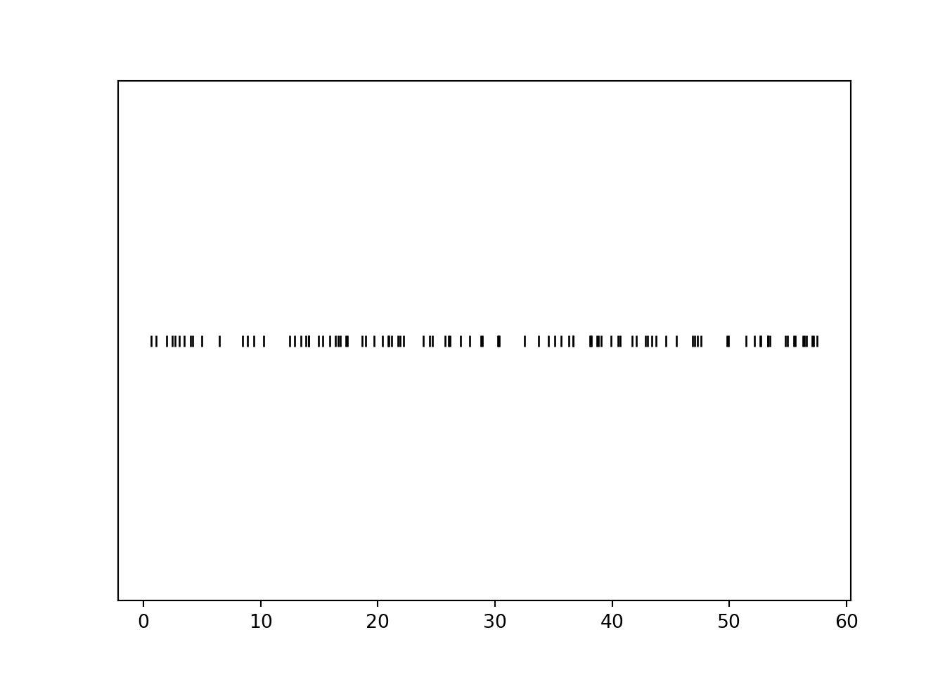

Calling .plot() (without 'rug') for simulated values of a continuous random variable produces a histogram, which we will discuss in much more detail in Chapter 5.

plt.figure()
R.sim(10000).plot()
plt.show()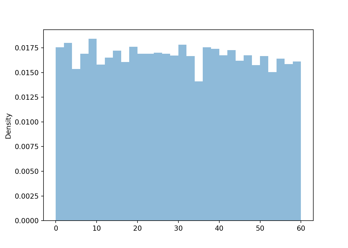

We can simulate and plot many $(R, Y)$ pairs of arrival times; compare to Figure 3.6 (without the rug).

(R & Y).sim(1000).plot()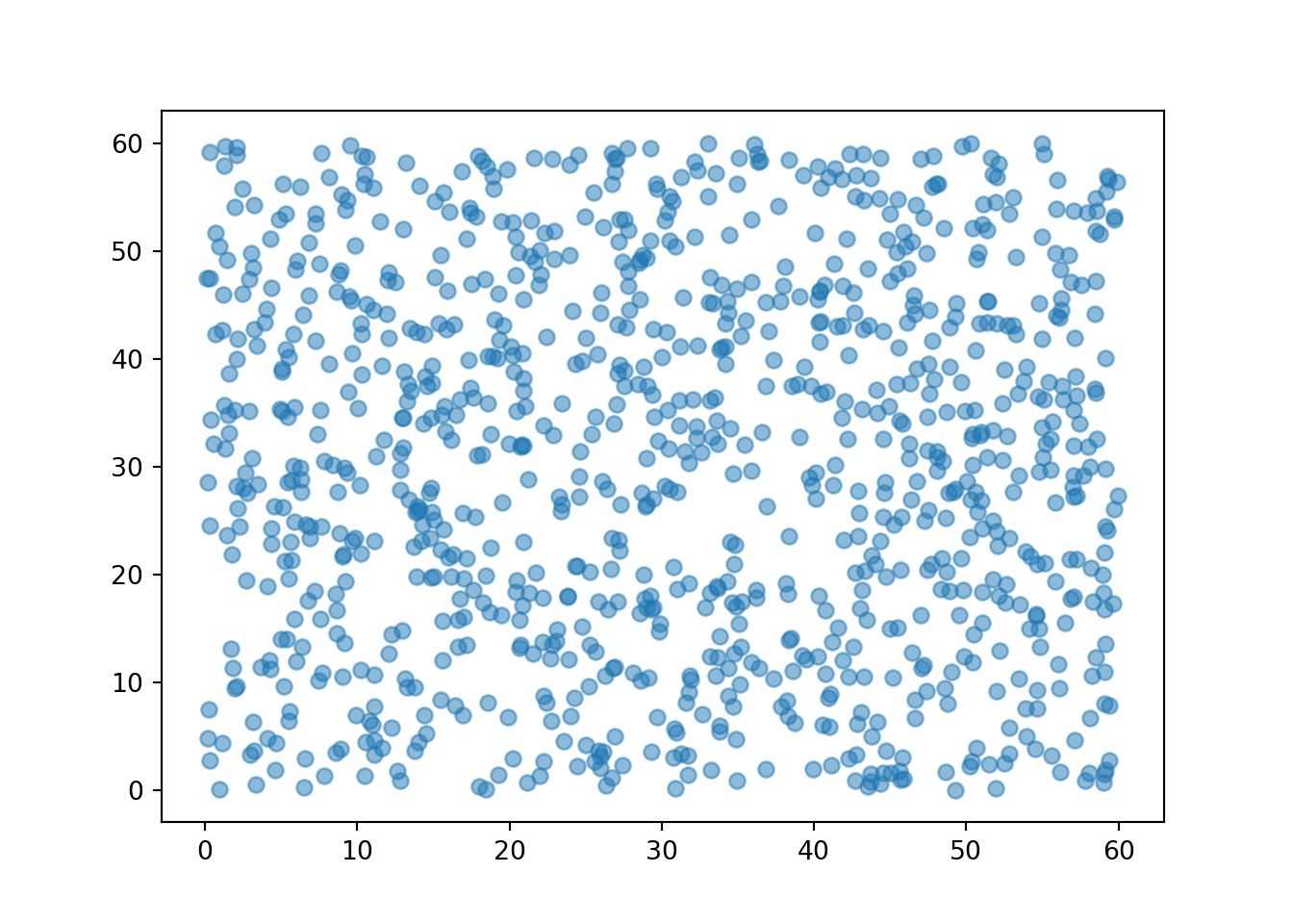

When plotting simulated pairs, the first component is plotted on the horizontal axis and the second component on the vertical axis. In the following plots, we’ll import matplotlib.pyplot as plt and use plt.xlabel("x-axis text") and plt.ylabel("y-axis text")to label axes.

We can also simulate and plot many $(T, W)$ pairs. For purposes of illustration, first we simulate all four random variables, then we’ll select the columns corresponding to $(T, W)$ and plot the simulated pairs.

import matplotlib.pyplot as plt

meeting_sim = (R & Y & T & W).sim(1000)

meeting_sim[2, 3].plot()
plt.xlabel("T")
plt.ylabel("W")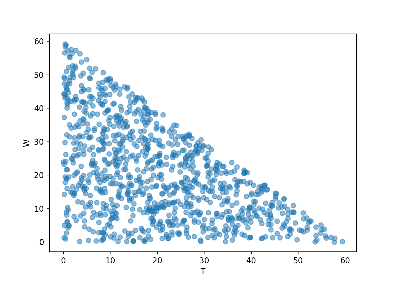

3.4.2 Independent Normal model

Now consider a Normal(30, 10) model, represented by the spinner in Figure 3.7.

Normal(mean = 30, sd = 10).sim(10)

Index	Result
0	34.36699251591295
1	29.89272408014123
2	24.8798074009082
3	35.301076397298964
4	28.8018551220353
5	47.48197369787165
6	26.854094099759507
7	8.308056591569411
8	20.379975189583355
...	...
9	20.531908737795742

We define a probability space corresponding to (Regina, Cady) pairs of arrival times, by assuming that their arrival times individually follow a Normal(30, 10) model, independently of each other. That is, we spin the Normal(30, 10) spinner twice to simulate a pair of arrival times.

P = Normal(30, 10) ** 2
P.sim(10)

Index	Result
0	(25.526952819232772, 53.647177301416534)
1	(45.08057146131936, 28.62561851066699)
2	(37.796876490441065, 5.507396181169753)
3	(30.4219475320437, 44.51715619922504)
4	(21.50862136658064, 18.9859393379374)
5	(50.6503483781549, 27.26018749676494)
6	(37.4284527786448, 25.09526760977524)
7	(52.644707931, 42.96655543076358)
8	(6.02564107384978, 24.04219601089075)
...	...
9	(22.738540578815865, 25.325180612776798)

We can unpack the individual $R$, $Y$ random variables and define $W$, $T$ as before.

R, Y = RV(P)

W = abs(R - Y)

T = (R & Y).apply(min)

We can simulate values of $R$ and plot them along a number line in a rug plot; compare to Figure 3.8. (Technically, the Normal(30, 10) assigns small but positive probability to values outside of [0, 60], so we might see some values outside of [0, 60].)

plt.figure()
R.sim(100).plot('rug')
plt.show()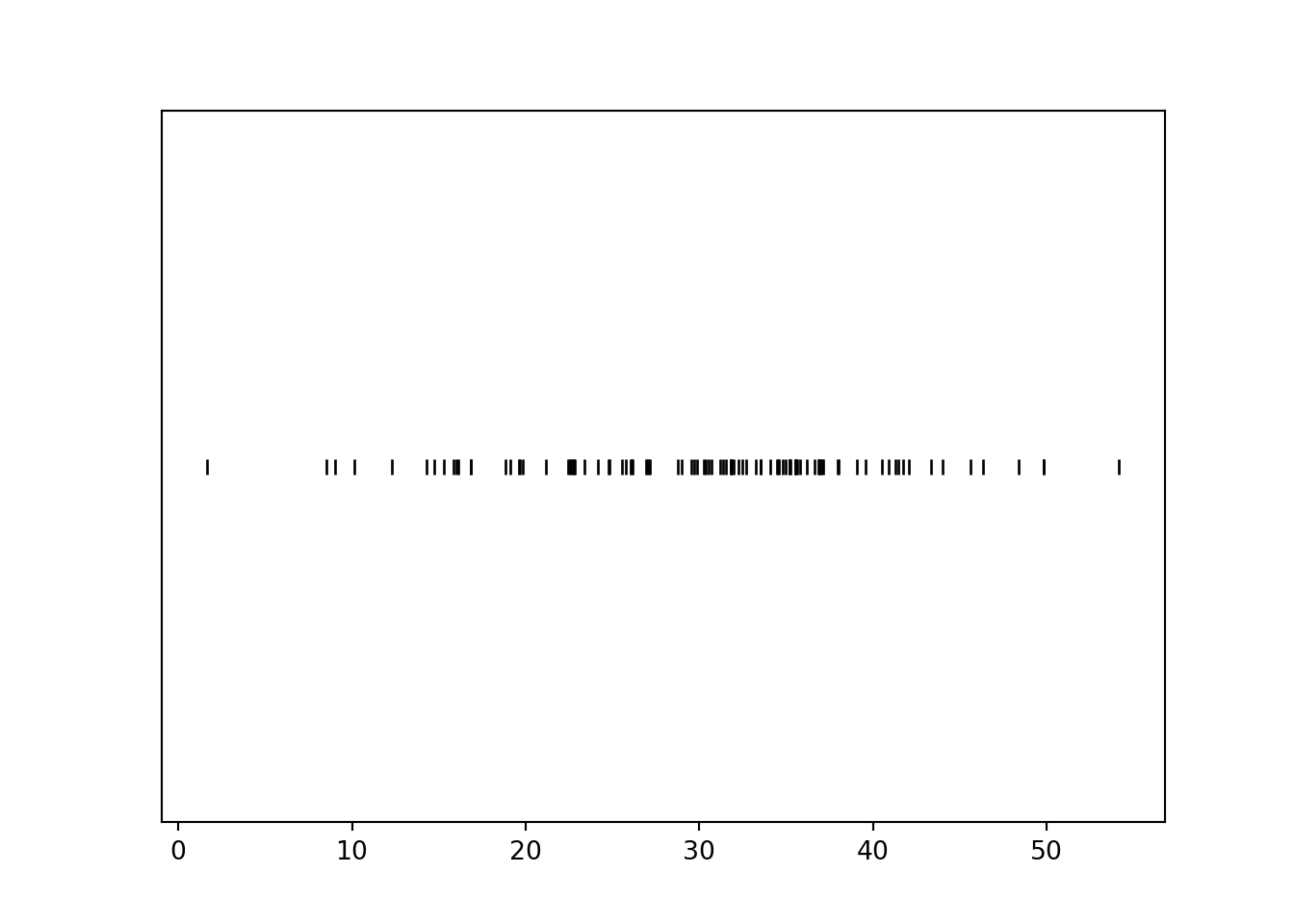

We can simulate many values and summarize them in a histogram. We’ll discuss histograms in more detail later, but notice that the histogram conveys that for a Normal(30, 10) distribution values near 30 are more likely than values near 0 or 60.

plt.figure()
R.sim(10000).plot()
plt.show()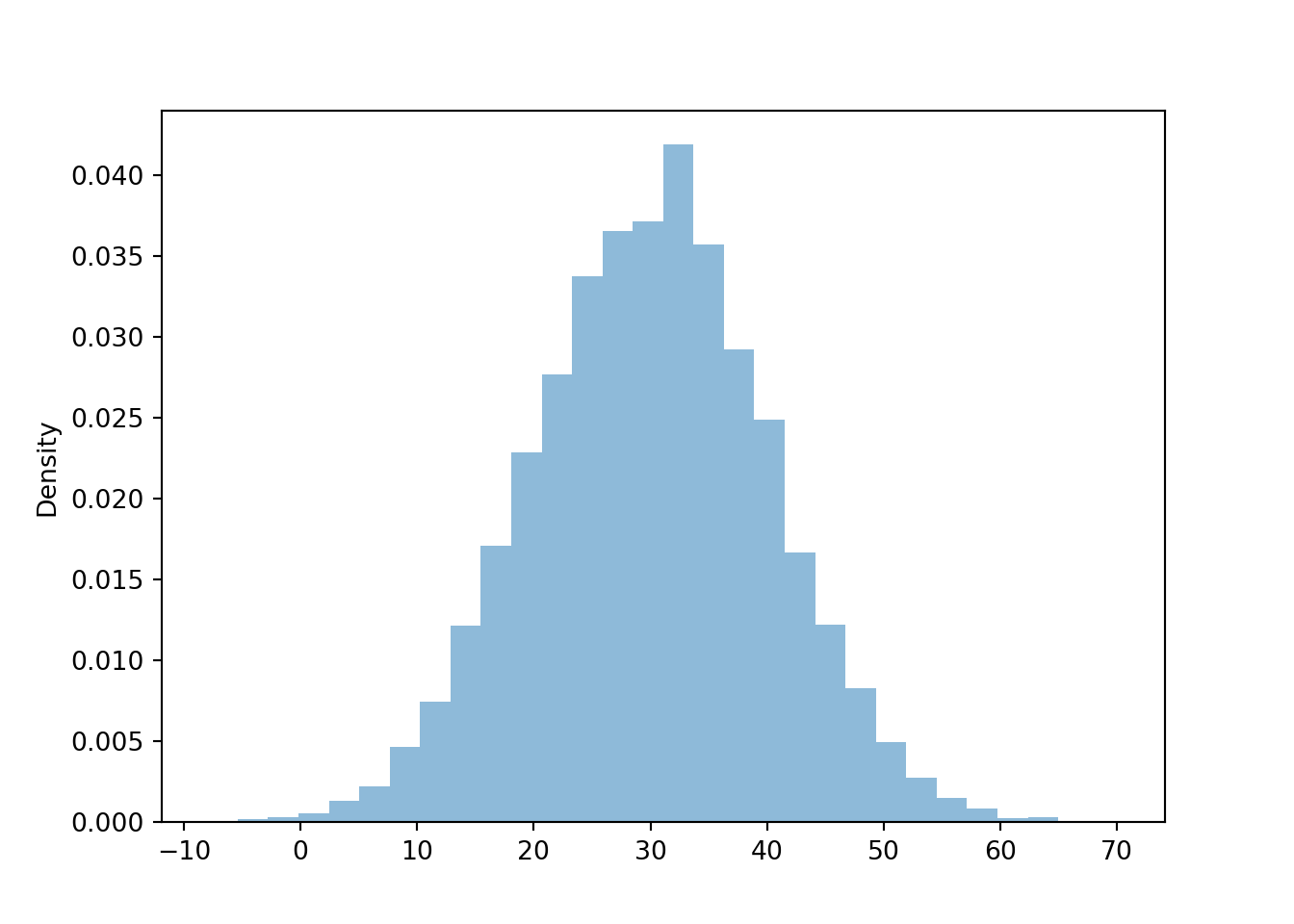

We can simulate and plot many $(R, Y)$ pairs of arrival times; compare to Figure 3.10 (without the rug).

(R & Y).sim(1000).plot()
plt.xlabel("R");
plt.ylabel("Y");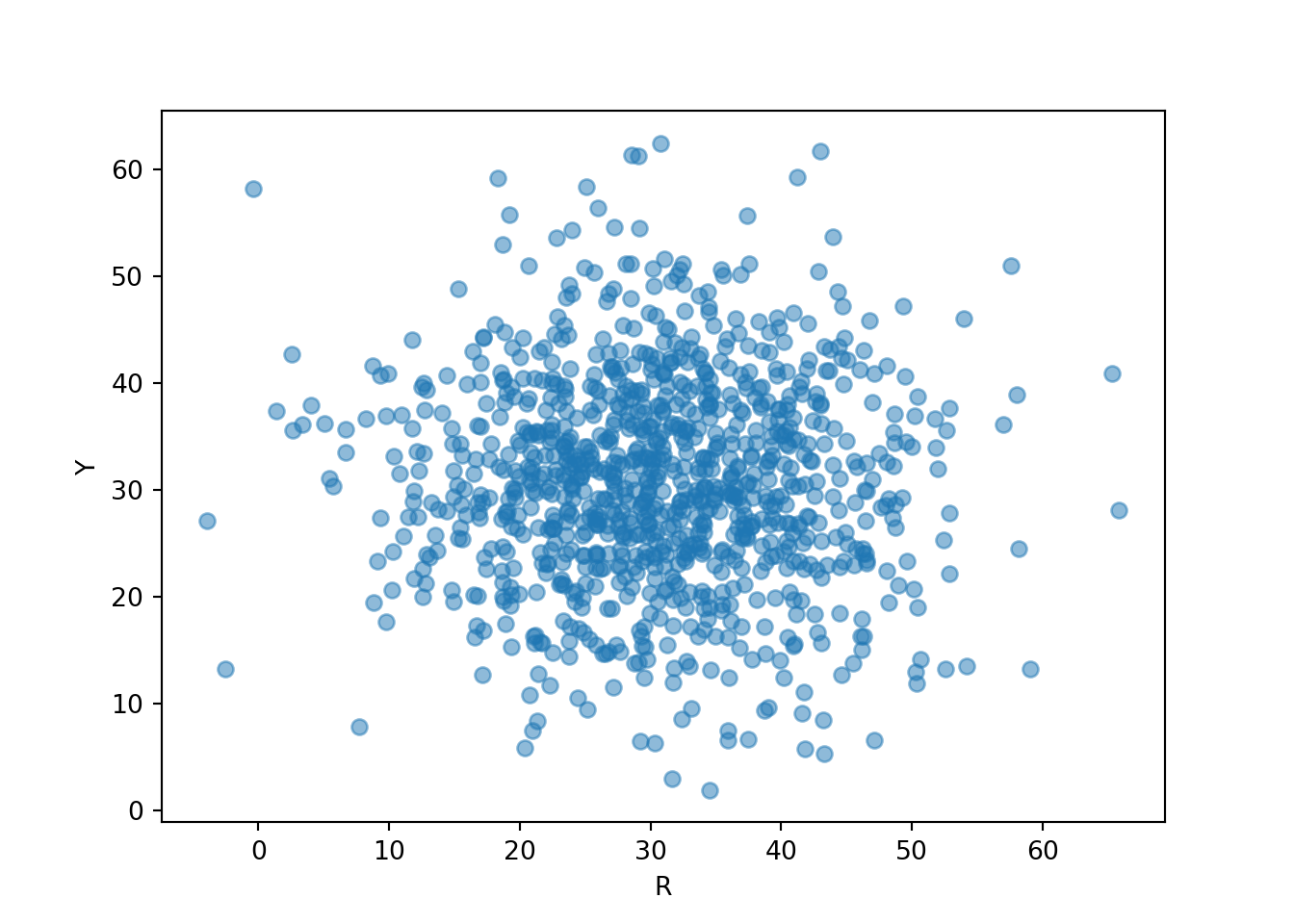

We can also simulate and plot many $(T, W)$ pairs. Notice that the plot looks quite different from the one for the independent Uniform(0, 60) model for arrival times.

meeting_sim = (R & Y & T & W).sim(1000)

meeting_sim[2, 3].plot()
plt.xlabel("T");
plt.ylabel("W");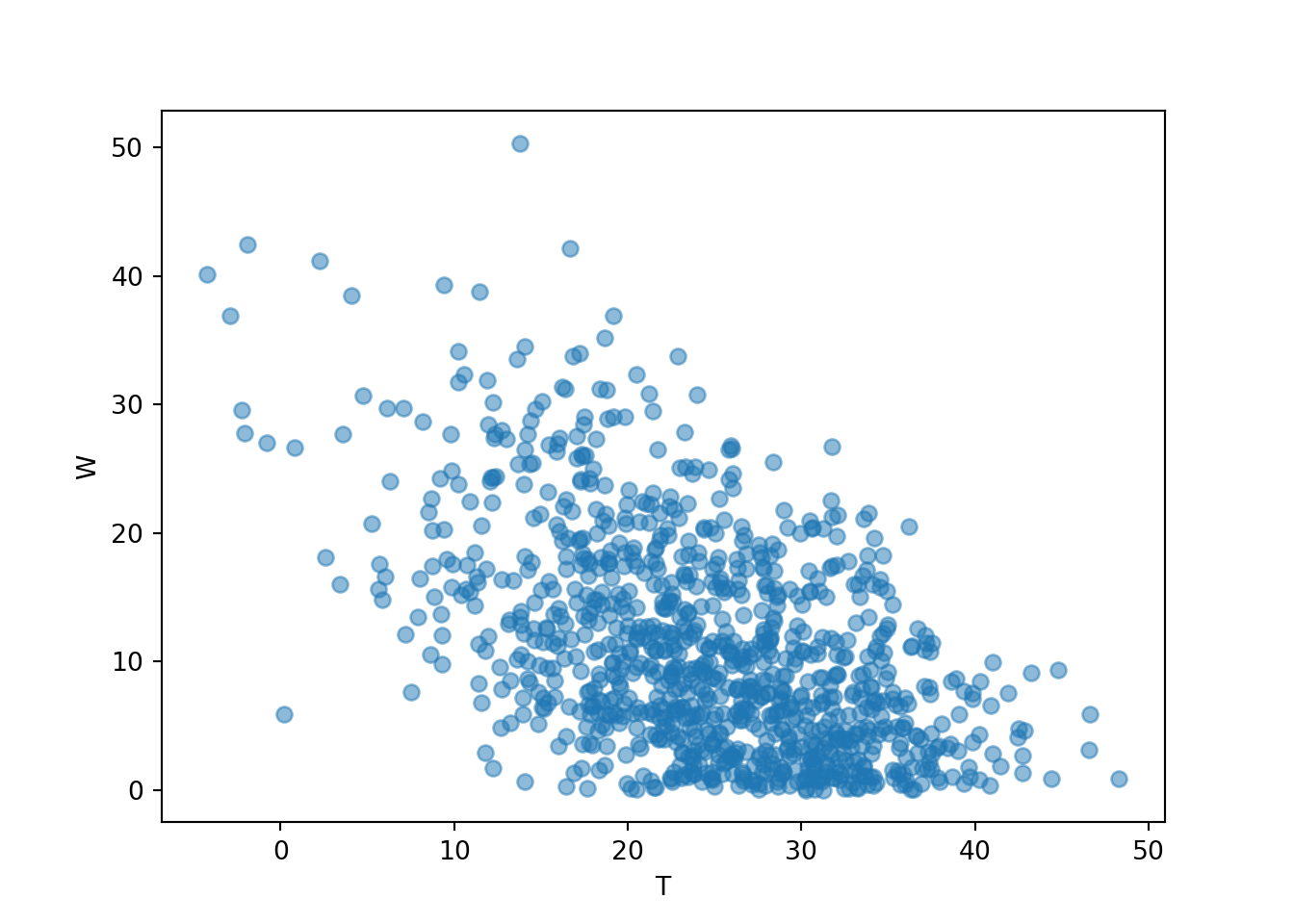

3.4.3 Bivariate Normal model

Now assume that Regina and Cady tend to arrive around the same time. We haven’t yet seen how to construct spinners to reflect dependence, but we’ll briefly introduce a particular model and some code. One way to model pairs of values that have a relationship or correlation is with a BivariateNormal model, like in the following.

P = BivariateNormal(mean1 = 30, sd1 = 10, mean2 = 30, sd2 = 10, corr = 0.7)
P.sim(10)

Index	Result
0	(46.29377271361334, 44.6617485721662)
1	(30.846072113770294, 27.371379313173115)
2	(23.7199274511314, 20.684000458988073)
3	(47.55476646762313, 46.727024440633)
4	(23.97205215354839, 41.52565999176303)
5	(19.540536182268667, 21.728970573940728)
6	(36.24164963838549, 36.31883895118515)
7	(56.677365937065986, 47.43571287106073)
8	(35.70420911719464, 43.172942419694785)
...	...
9	(25.357373758412162, 24.328108021694153)

Note that a BivariateNormal probability space returns pairs directly. We can unpack the pairs as before, and plot some simulated values.

R, Y = RV(P)

(R & Y).sim(1000).plot()
plt.xlabel("R");
plt.ylabel("Y");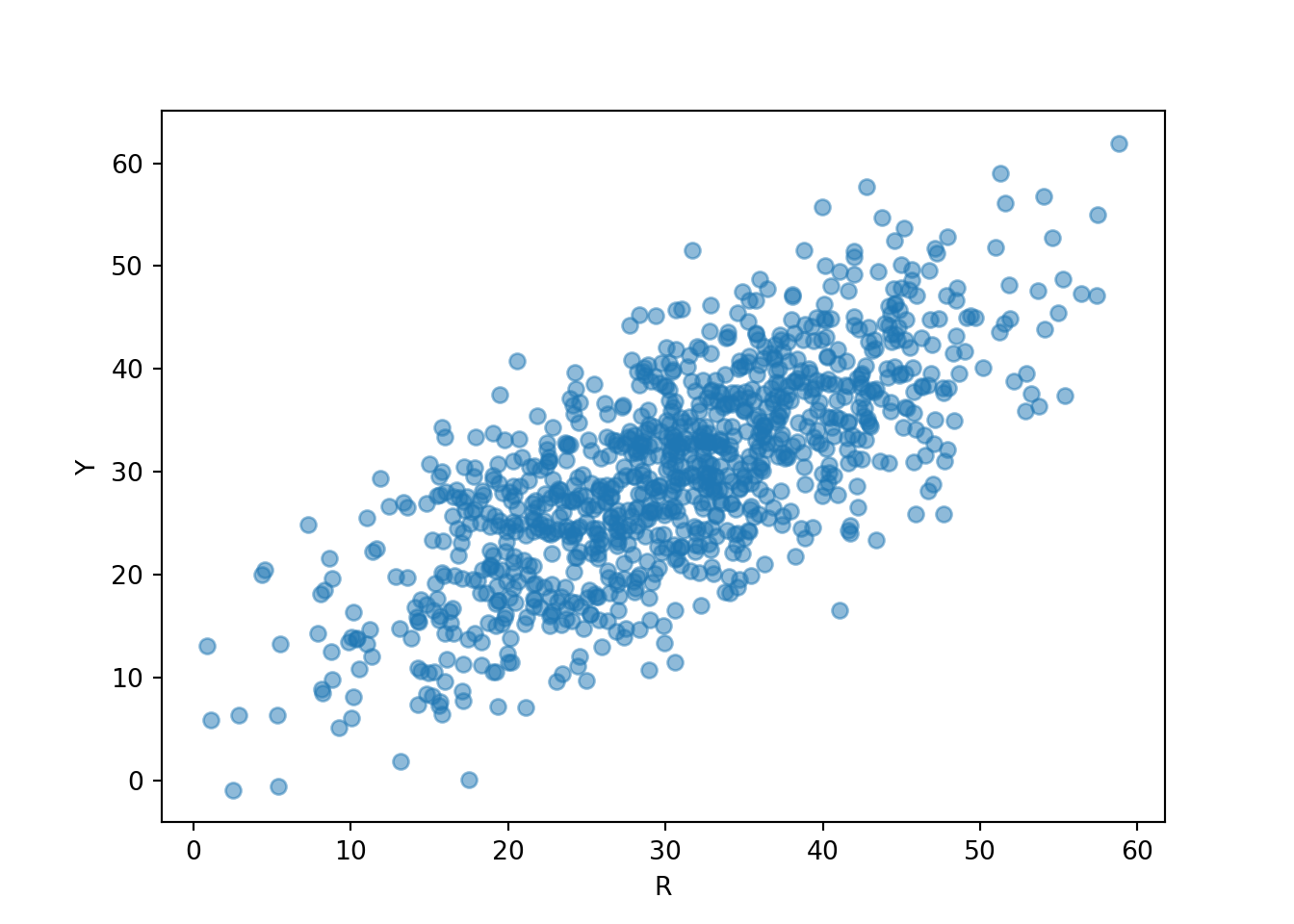

Now we see that Regina and Cady tend to arrive near the same time, similar to Figure 2.15.

If we plot $(T, W)$ pairs, we expect values of the waiting time $W$ to tend to be closer to 0 than in the independent arrivals models. Compare the scale on the vertical axis, corresponding to $W$, in each of the three plots of $(T, W)$ pairs in this section.

W = abs(R - Y)

T = (R & Y).apply(min)

meeting_sim = (R & Y & T & W).sim(1000)

meeting_sim[2, 3].plot()
plt.xlabel("T");
plt.ylabel("W");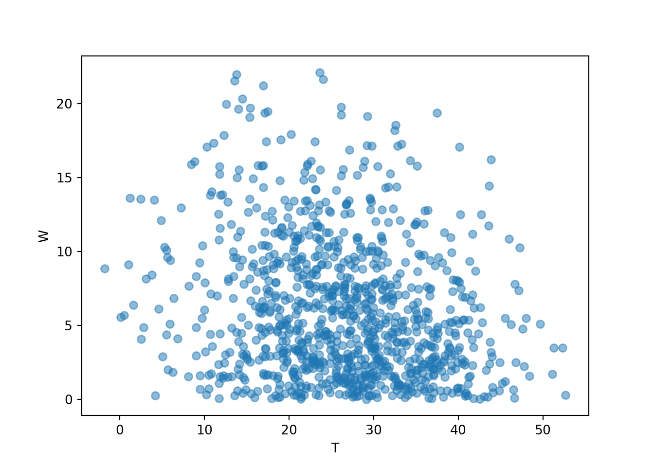

A call to sim always simulates independent repetitions from the model, but be careful about what this means. In the Bivariate Normal model, the $R$ and $Y$ values are dependent within a repetition. However, the $(R, Y)$ pairs are independent between repetitions. Thinking in terms of a table, the $R, Y$ columns are dependent, but the rows are independent.

We will study specific probability models like Normal and BivariateNormal in much more detail as we go.

3.4.4 Exercises

Exercise 3.10 Write Symbulate code to conduct the simulation in Exercise 3.4. Caveat: don’t worry about the code to discard repetitions where the dart lands off the board. (We’ll return to this later.)

Exercise 3.11 Consider a continuous version of the dice rolling problem where instead of rolling two fair four-sided dice (which return values 1, 2, 3, 4) we spin twice a Uniform(1, 4) spinner (which returns any value in the continuous range between 1 and 4). Let $X$ be the sum of the two spins and let $Y$ be the larger of the two spins. Write Symbulate code to define an appropriate probability space and random variables, and simulate a few repetitions.

3.5 Approximating probabilities: Relative frequencies

We can use simulation-based relative frequencies to approximate probabilities. That is, the probability of event $A$ can be approximated by simulating—according to the assumptions encoded in the probability measure $\textrm{P}$—the random phenomenon a large number of times and computing the relative frequency of $A$.

\[ {\small \textrm{P}(A) \approx \frac{\text{number of repetitions on which $A$ occurs}}{\text{number of repetitions}}, \quad \text{for a large number of repetitions simulated according to $\textrm{P}$} } \]

In practice, many repetitions of a simulation are performed on a computer to approximate what happens in the “long run”. However, we often start by carrying out a few repetitions by hand to help make the process more concrete.

Example 3.5 Recall your simulation results from Example 3.1; ours are in Table 3.1. Based only on your 10 repetitions, how would you approximate the following? (Don’t worry if the approximations are any good yet.)

$\textrm{P}(A)$, where $A$ is the event that the first roll is 3.
$\textrm{P}(X=6)$
$\textrm{P}(X \ge 6)$
$\textrm{P}(Y = 3)$
$\textrm{P}(Y \ge 3)$
$\textrm{P}(X=6, Y=3)$
$\textrm{P}(X\ge6, Y \ge 3)$

Solution (click to expand)

Solution 3.5. See Table 3.1 for the results of our simulation.

Approximate $\textrm{P}(A)$ by 4/10 = 0.4, the relative frequency of event $A$ in the simulation; that is, the proportion of repetitions where the first roll is 3.
Approximate $\textrm{P}(X=6)$ by 2/10 = 0.2, the proportion of repetitions where the sum is 6.
Approximate $\textrm{P}(X\ge 6)$ by 5/10 = 0.5, the proportion of repetitions where the sum is at least 6.
Approximate $\textrm{P}(Y=3)$ by 3/10 = 0.3, the proportion of repetitions where the max is 3.
Approximate $\textrm{P}(Y\ge 3)$ by 7/10 = 0.7, the proportion of repetitions where the max is at least 3.
Approximate $\textrm{P}(X=6, Y = 3)$ by 1/10 = 0.1, the proportion of repetitions where both the sum is 6 and the max is 3.
Approximate $\textrm{P}(X\ge 6, Y \ge 3)$ by 5/10 = 0.5, the proportion of repetitions where both the sum is at least 6 and the max is at least 3. (Since $X\ge 6$ implies $Y\ge 3$, $\textrm{P}(X\ge 6, Y\ge 3) = \textrm{P}(X\ge 6)$.)

Example 3.6 Continuing Example 3.5.

Construct a table of the simulated relative frequencies of each possible value $x$ of $X$.
Construct a table of the simulated relative frequencies of each possible value $(x, y)$ pair of $(X, Y)$.

Solution (click to expand)

Solution 3.6. For discrete random variables like these we can make tables or plots summarizing the observed values of the random variables and their corresponding relative frequencies.

Summarizing our simulation results from Table 3.1, the observed values of $X$ and corresponding relative frequencies are

$x$	Relative frequency
2	1/10
3	2/10
4	0
5	2/10
6	2/10
7	3/10
8	0

The above table¹⁸ represents an approximation of the distribution of $X$, albeit a bad approximation; compare with Table 2.14.

We can summarize simulated $(X, Y)$ pairs and their relative frequencies, as in the following two-way table; compare with Table 2.17.

$x, y$	1	2	3	4
2	1/10	0	0	0
3	0	2/10	0	0
4	0	0	0	0
5	0	0	2/10	0
6	0	0	1/10	1/10
7	0	0	0	3/10
8	0	0	0	0

You might have noticed that many of the simulated relative frequencies in Example 3.5 provide terrible estimates of the corresponding probabilities. For example, the true probability that the first roll is a 3 is $\textrm{P}(A) = 0.25$ while the simulated relative frequency is 0.4. The problem is that the simulation only consisted of 10 repetitions. Probabilities can be approximated by long run relatively frequencies, but 10 repetitions certainly doesn’t qualify as the long run! The more repetitions we perform the better our estimates should be. But how many repetitions is sufficient? And how accurate are the estimates? We will address these issues in Section 3.6.

3.5.1 A few Symbulate commands for summarizing simulation output

We’ll continue with the dice rolling example. Recall the setup.

P = DiscreteUniform(1, 4) ** 2

X = RV(P, sum)

Y = RV(P, max)

First we’ll simulate and store 10 values of $X$.

x = X.sim(10)
x # displays the simulated values

Index	Result
0	7
1	3
2	2
3	5
4	5
5	8
6	5
7	4
8	6
...	...
9	5

Suppose we want to find the relative frequency of 6. We can count the number of simulated values equal to 6 with count_eq().

x.count_eq(6)

The count is the frequency. To find the relative frequency we simply divide by the number of simulated values.

x.count_eq(6) / 10

0.1

We can find frequencies of other events using the “count” functions:

count_eq(u): count equal to ($=$) u
count_neq(u): count not equal to ($\neq$) u
count_leq(u): count less than or equal to ($\le$) u
count_lt(u): count less than ($<$) u
count_geq(u): count greater than or equal to ($\ge$) u
count_gt(u): count greater than ($>$) u
count: count according to a custom True/False criteria (see examples below)

Using count() with no inputs to defaults to “count all”, which provides a way to count the total number of simulated values. (This is especially useful when conditioning.)

x.count_eq(6) / x.count()

0.1

The tabulate method provides a quick summary of the individual simulated values and their frequencies.

x.tabulate()

Value	Frequency
2	1
3	1
4	1
5	4
6	1
7	1
8	1
Total	10

By default, tabulate returns frequencies (counts). Adding the argument¹⁹ normalize = True returns relative frequencies (proportions).

x.tabulate(normalize = True)

Value	Relative Frequency
2	0.1
3	0.1
4	0.1
5	0.4
6	0.1
7	0.1
8	0.1
Total	1.0

We often initially simulate a small number of repetitions to see what the simulation is doing and check that it is working properly. However, in order to accurately approximate probabilities or distribution we simulate a large number of repetitions (usually thousands for our purposes). Now let’s simulate many $X$ values and summarize the results.

x = X.sim(10000)

x.tabulate(normalize = True)

Table 3.8: Table representing simulation-based approximate distribution of $X$, the sum of two rolls of a fair four-sided die.

Value	Relative Frequency
2	0.062
3	0.122
4	0.1847
5	0.2475
6	0.1927
7	0.1261
8	0.065
Total	1.0

Compare to Table 2.14; with 10000 repetitions the simulation based approximations are pretty close to the theoretical probabilities.

Graphical summaries play an important role in analyzing simulation output. We have previously seen rug plots of individual simulated values. Rug plot emphasize that realizations of a random variable are numbers along a number line. However, a rug plot does not adequately summarize relative frequencies. Instead, calling .plot() for simulated values of a discrete random variable produces²⁰ an impulse plot which displays the simulated values and their relative frequencies; see Figure 3.11 and compare to Figure 2.16. Since we stored the simulated values as x, the same simulated values are used to produce Table 3.8 and Figure 3.11.

x.plot()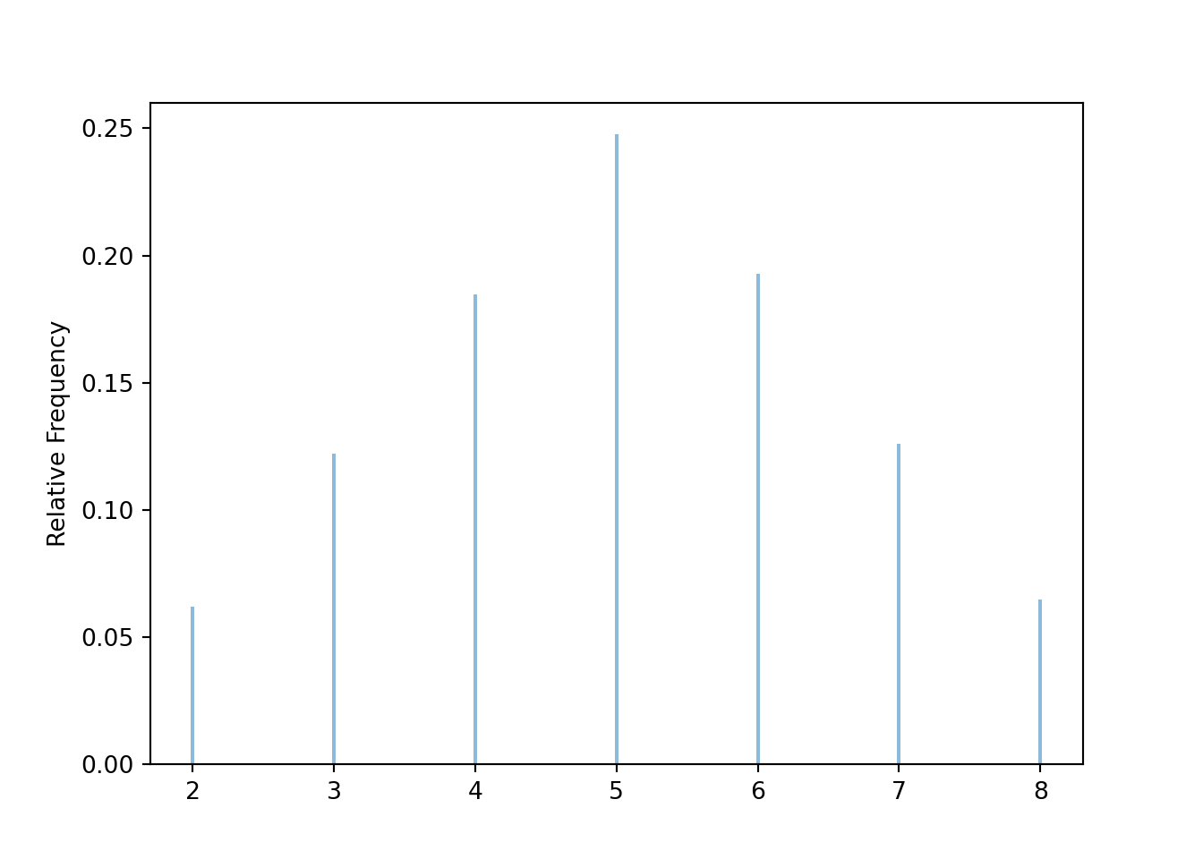

Figure 3.11: Impulse plot representing simulation-based approximate distribution of $X$, the sum of two rolls of a fair four-sided die.

Now we simulate and summarize a few $(X, Y)$ pairs.

x_and_y = (X & Y).sim(10)
x_and_y

Index	Result
0	(6, 4)
1	(3, 2)
2	(4, 3)
3	(4, 3)
4	(8, 4)
5	(4, 2)
6	(2, 1)
7	(4, 2)
8	(3, 2)
...	...
9	(8, 4)

Pairs of values can also be tabulated.

x_and_y.tabulate()

Value	Frequency
(2, 1)	1
(3, 2)	2
(4, 2)	2
(4, 3)	2
(6, 4)	1
(8, 4)	2
Total	10

x_and_y.tabulate(normalize = True)

Value	Relative Frequency
(2, 1)	0.1
(3, 2)	0.2
(4, 2)	0.2
(4, 3)	0.2
(6, 4)	0.1
(8, 4)	0.2
Total	1.0

Individual pairs can be plotted in a scatter plot, which is a two-dimensional analog of a rug plot.

x_and_y.plot()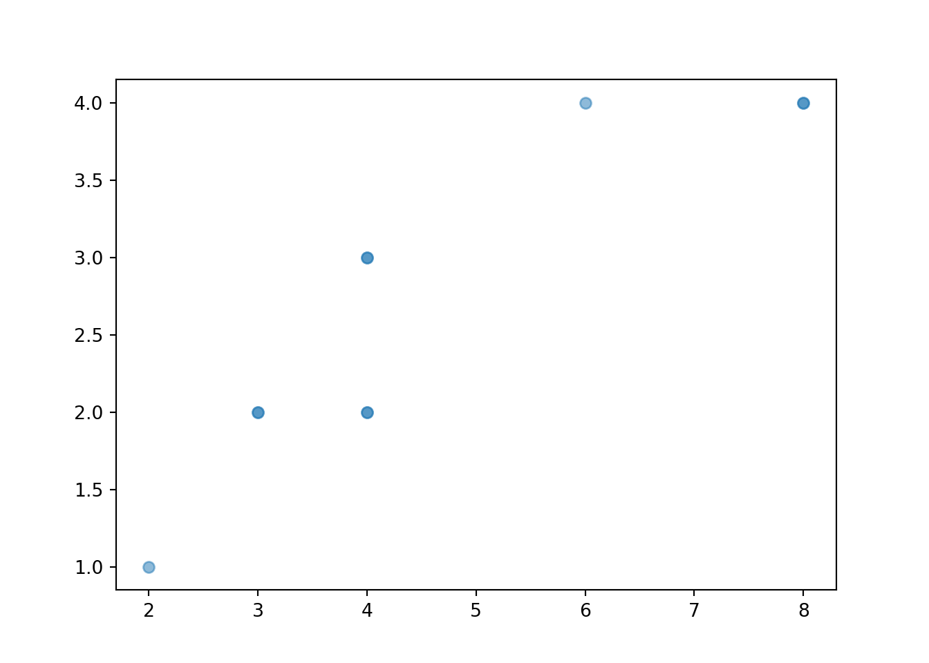

The values can be “jittered” slightly, as below, so that points do not coincide.

x_and_y.plot(jitter = True)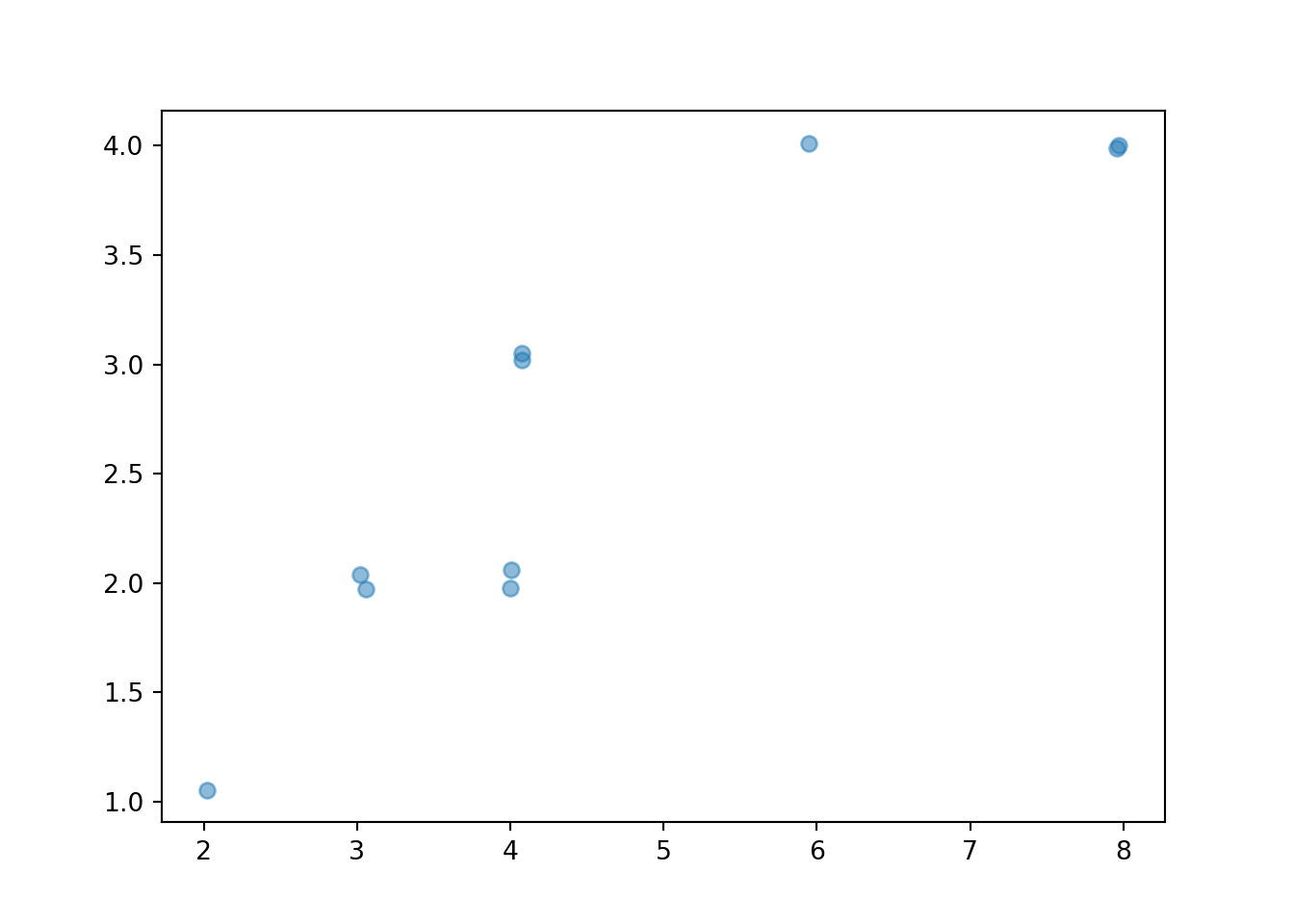

The two-dimensional analog of an impulse plot is a tile plot. For two discrete variables, the 'tile' plot type produces a tile plot (a.k.a. heat map) where rectangles represent the simulated pairs with their relative frequencies visualized on a color scale.

x_and_y.plot('tile')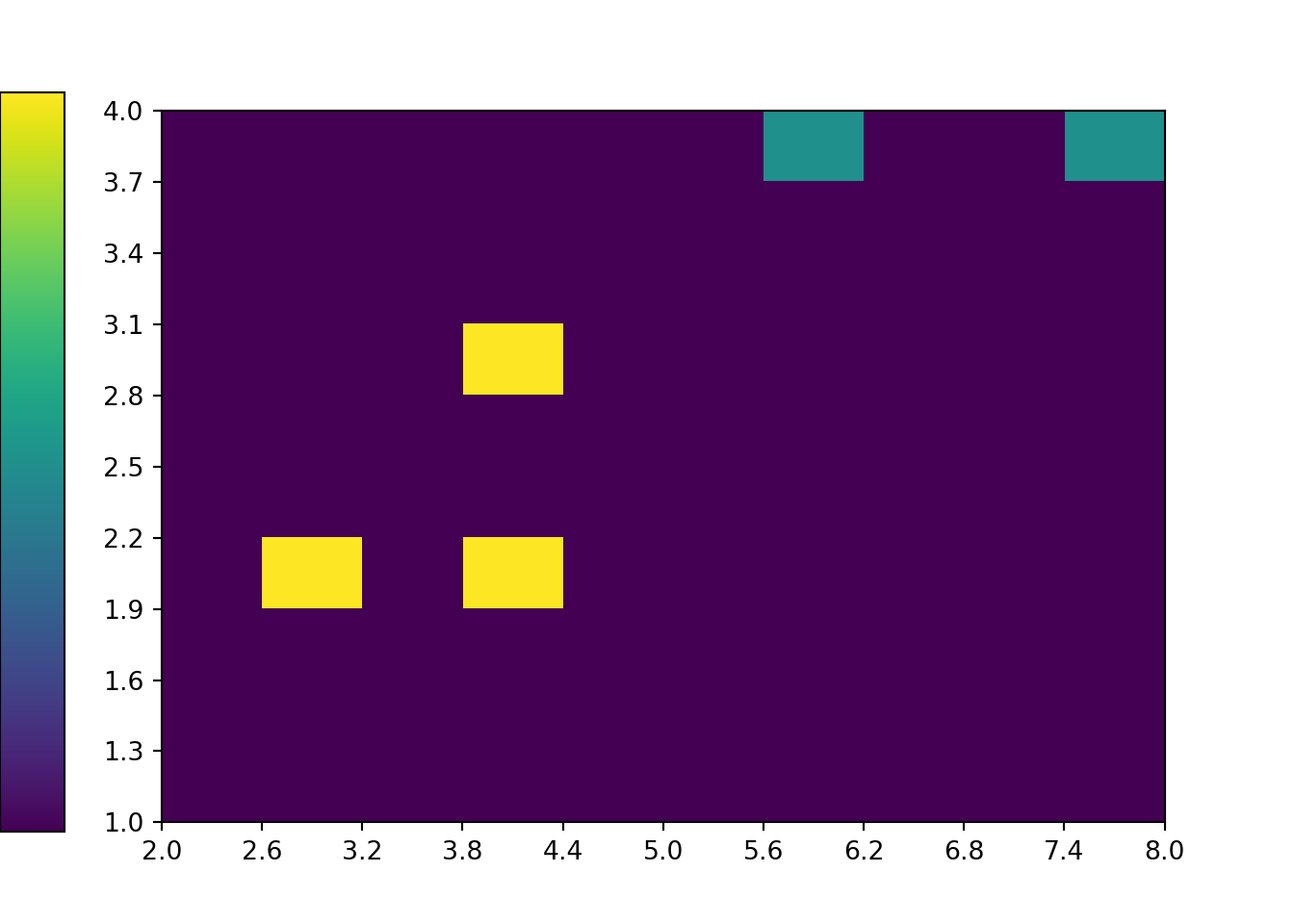

Custom functions can be used with count to compute relative frequencies of events involving multiple random variables. Suppose we want to approximate $\textrm{P}(X<6, Y \ge 2)$. We first define a Python function which takes as an input a pair u = (u[0], u[1]) and returns True if u[0] < 6 and u[1] >= 2.


def is_x_lt_6_and_y_ge_2(u):
  if u[0] < 6 and u[1] >= 2:
    return True
  else:
    return False

Now we can use this function along with count to find the simulated relative frequency of the event $\{X <6, Y \ge 2\}$. Remember that x_and_y stores $(X, Y)$ pairs of values, so the first coordinate x_and_y[0] represents values of $X$ and the second coordinate x_and_y[1] represents values of $Y$.

x_and_y.count(is_x_lt_6_and_y_ge_2) / x_and_y.count()

0.6

We could also count use Boolean logic; basically using indicators and the property $\textrm{I}_{\{X<6,Y\ge 2\}}=\textrm{I}_{\{X<6\}}\textrm{I}_{\{Y\ge 2\}}$.

((x_and_y[0] < 6) * (x_and_y[1] >= 2)).count_eq(True) / x_and_y.count()

0.6

Now we simulate many $(X, Y)$ pairs and summarize their frequencies.

x_and_y = (X & Y).sim(10000)

x_and_y.tabulate()

Value	Frequency
(2, 1)	646
(3, 2)	1202
(4, 2)	601
(4, 3)	1275
(5, 3)	1277
(5, 4)	1239
(6, 3)	651
(6, 4)	1247
(7, 4)	1232
(8, 4)	630
Total	10000

Here are the relative frequencies; compare with Table 2.16.

x_and_y.tabulate(normalize = True)

Value	Relative Frequency
(2, 1)	0.0646
(3, 2)	0.1202
(4, 2)	0.0601
(4, 3)	0.1275
(5, 3)	0.1277
(5, 4)	0.1239
(6, 3)	0.0651
(6, 4)	0.1247
(7, 4)	0.1232
(8, 4)	0.063
Total	1.0

When there are thousands of simulated pairs, a scatter plot does not adequately display relative frequencies, even with jittering.

x_and_y.plot(jitter = True)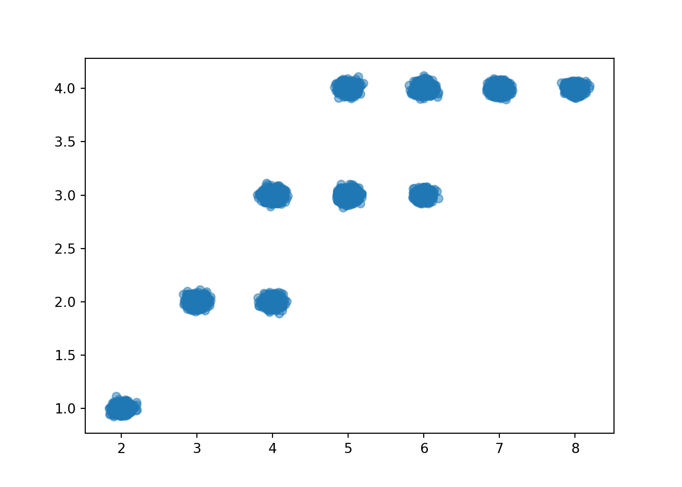

The tile plot provides a better summary. Notice how the colors represent the relative frequencies in the previous table.

x_and_y.plot('tile')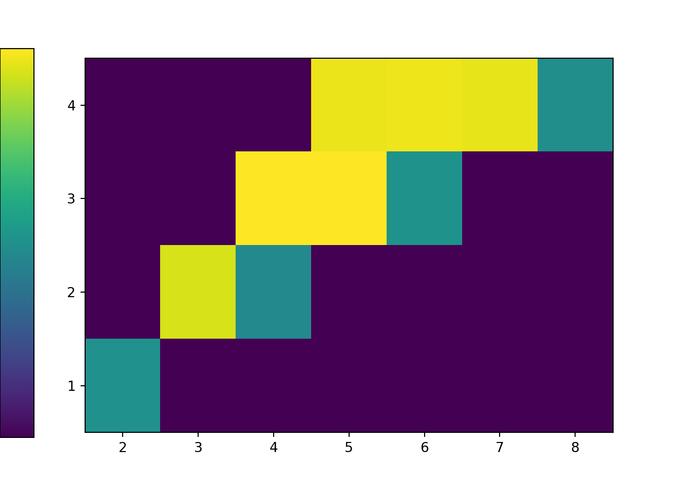

Finally, we find the simulated relative frequency of the event $\{X <6, Y \ge 2\}$.

x_and_y.count(is_x_lt_6_and_y_ge_2) / x_and_y.count()

0.5594

3.5.2 Approximating probabilities in the meeting problem

Example 3.7 Recall the independent Uniform(0, 60) model for arrival times of Example 3.3. Use the simulation results in Table 3.3 to approximate the following. (Don’t worry if the approximations are any good yet.)

$\textrm{P}(T < 15)$
$\textrm{P}(W < 15)$
$\textrm{P}(T < 15, W < 15)$
$\textrm{P}(R = 20)$
$\textrm{P}(19.5 < R < 20.5)$

Solution (click to expand)

Solution 3.7.

Approximate $\textrm{P}(T < 15)$ by 3/10 = 0.3, the proportion of repetitions where the first arrival time is less than 15 minutes.
Approximate $\textrm{P}(W < 15)$ by 6/10 = 0.6, the proportion of repetitions where the waiting time is less than 15 minutes.
Approximate $\textrm{P}(T < 15, W < 15)$ by 2/10 = 0.2, the proportion of repetitions where both the first arrival time and the waiting time are less than 15 minutes.
Approximate $\textrm{P}(R=20)$ by 0, the proportion of repetitions where $R$ is equal to 20.
Approximate $\textrm{P}(19.5 < R < 20.5)$ by 1/10 = 0.1, the proportion of repetitions where $R$, rounded to the nearest minute, is equal to 20.

An event either happens or not. Regardless of whether an event involves a discrete or continuous random variable, the probability of the event is approximated in the same way. However, the kinds of events we’re interested in differ between those involving discrete and those involving continuous random variables. The probability that a continuous random variable is equal to any particular value is 0, so we’re not interested in approximating “equals to” probabilities for continuous random variables. When dealing with continuous random variables in practice, “equals to” is really “close to”, and we compute approximate “close to” probabilities with relative frequencies are usual. (Later, we’ll see what it means to condition on a continuous random variable being equal to some value.)

To get better approximations for the probabilities in Example 3.3 we would need to simulate many more repetitions. But the process of approximating probabilities with simulated relative frequencies is the same as in Example 3.3.

Simulation can also be used to investigate how sensitive (approximate) probabilities are to changes in assumptions.

Example 3.8 Write Symbulate code to run simulations and use the results to approximate the probability that Regina and Cady arrive with 15 minutes of each other for each of the three models in Section 3.4.

Independent Uniform model
Independent Normal model
Bivariate Normal model

Solution (click to expand)

Solution 3.8. There are a few ways to code this, but one way is to define the waiting time random variable $W=|R-Y|$ and find simulated relative frequencies of the event $\{W<15\}$.

First the independent Uniform model.

P = Uniform(0, 60) ** 2
R, Y = RV(P)

W = abs(R - Y)

w = W.sim(10000)

w.count_lt(15) / w.count()

0.4344

Next the independent Normal model.

P = Normal(30, 10) ** 2
R, Y = RV(P)

W = abs(R - Y)

w = W.sim(10000)

w.count_lt(15) / w.count()

0.7167

Finally, the Bivariate Normal model.

P = BivariateNormal(mean1 = 30, sd1 = 10, mean2 = 30, sd2 = 10, corr = 0.7)
R, Y = RV(P)

W = abs(R - Y)

w = W.sim(10000)

w.count_lt(15) / w.count()

0.9467

We see that these changes in assumptions have substantial influence on this probability. The simulations shows that they are roughly 1.7 times more likely to arrive within 15 minutes of each other under the independent Normal model than under the independent Uniform model, and roughly 1.3 times more likely under the Bivariate Normal model than under the independent Normal model.

We have previously seen rug plots of individual simulated values. Rug plot emphasize that realizations of a random variable are numbers along a number line. However, a rug plot does not adequately summarize the distribution of values. Instead, calling .plot() for simulated values of a continuous random variable produces a histogram.

plt.figure()
w.plot()
plt.show()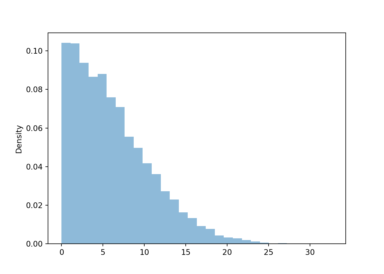

We will cover histograms and marginal distributions of continuous random variables in much more detail in Chapter 5.

3.5.3 Exercises

Exercise 3.12 The latest series of collectible Lego Minifigures contains 3 different Minifigure prizes (labeled 1, 2, 3). Each package contains a single unknown prize. Suppose we only buy 3 packages and we consider as our sample space outcome the results of just these 3 packages (prize in package 1, prize in package 2, prize in package 3). For example, 323 (or (3, 2, 3)) represents prize 3 in the first package, prize 2 in the second package, prize 3 in the third package. Let $X$ be the number of distinct prizes obtained in these 3 packages. Let $Y$ be the number of these 3 packages that contain prize 1.

Explain how you could, in principle, conduct a simulation by hand and use the results to approximate
1. $\textrm{P}(X = 2)$
2. $\textrm{P}(Y = 1)$
3. $\textrm{P}(X = 2, Y = 1)$
Write Symbulate code to conduct a simulation and approximate the values in part 1.
Write Sybulate code to conduct a simulation and approximate
1. Marginal distribution of $X$
2. Marginal distribution of $Y$
3. Joint distribution of $X$ and $Y$

Exercise 3.13 Repeat Exercise 3.12, but now assuming that 10% of boxes contain prize 1, 30% contain prize 2, and 60% contain prize 3.

Exercise 3.14 Maya is a basketball player who makes 40% of her three point field goal attempts. Suppose that at the end of every practice session, she attempts three pointers until she makes one and then stops. Let $X$ be the total number of shots she attempts in a practice session. Assume shot attempts are independent, each with probability of 0.4 of being successful.

Explain in words you could use simulation to approximate the distribution of $X$ and $\textrm{P}(X > 3)$.
Write Symbulate code to approximate the distribution of $X$ and $\textrm{P}(X > 3)$.

Exercise 3.15 Consider a continuous version of the dice rolling problem where instead of rolling two fair four-sided dice (which return values 1, 2, 3, 4) we spin twice a Uniform(1, 4) spinner (which returns any value in the continuous range between 1 and 4). Let $X$ be the sum of the two spins and let $Y$ be the larger of the two spins.

Describe in words how you could use simulation to approximate
1. $\textrm{P}(X < 3.5)$
2. $\textrm{P}(Y > 2.7)$
3. $\textrm{P}(X < 3.5, Y > 2.7)$
Write Symbulate code to conduct a simulation to approximate, via plots
1. the marginal distribution of $X$
2. the marginal distribution of $Y$
3. the joint distribution of $X$ and $Y$
4. The probabilities from part 1

3.6 Approximating probabilities: Simulation margin of error

The probability of an event can be approximated by simulating the random phenomenon a large number of times and computing the relative frequency of the event. After enough repetitions we expect the simulated relative frequency to be close to the true probability, but there probably won’t be an exact match. Therefore, in addition to reporting the approximate probability, we should also provide a margin of error which indicates how close we think our simulated relative frequency is to the true probability.

Section 1.2.1 introduced the relative frequency interpretation in the context of flipping a fair coin. After many flips of a fair coin, we expect the proportion of flips resulting in H to be close to 0.5. But how many flips is enough? And how “close” to 0.5? We’ll investigate these questions now.

Consider Figure 3.12 below. Each dot represents a set of 10,000 fair coin flips. There are 100 dots displayed, representing 100 different sets of 10,000 coin flips each. For each set of flips, the proportion of the 10,000 flips which landed on head is recorded. For example, if in one set 4973 out of 10,000 flips landed on heads, the proportion of heads is 0.4973. The plot displays 100 such proportions; similar values have been “binned” together for plotting. We see that 98 of these 100 proportions are between 0.49 and 0.51, represented by the blue dots. So if “between 0.49 and 0.51” is considered “close to 0.5”, then yes, in 10000 coin flips we would expect²¹ the proportion of heads to be close to 0.5.

$data
      phat  ci_lb  ci_ub good_ci
1   0.4973 0.4873 0.5073    TRUE
2   0.4999 0.4899 0.5099    TRUE
3   0.4996 0.4896 0.5096    TRUE
4   0.5000 0.4900 0.5100    TRUE
5   0.5044 0.4944 0.5144    TRUE
6   0.4970 0.4870 0.5070    TRUE
7   0.5001 0.4901 0.5101    TRUE
8   0.5083 0.4983 0.5183    TRUE
9   0.5087 0.4987 0.5187    TRUE
10  0.5002 0.4902 0.5102    TRUE
11  0.5029 0.4929 0.5129    TRUE
12  0.4984 0.4884 0.5084    TRUE
13  0.4938 0.4838 0.5038    TRUE
14  0.4974 0.4874 0.5074    TRUE
15  0.4997 0.4897 0.5097    TRUE
16  0.5061 0.4961 0.5161    TRUE
17  0.5040 0.4940 0.5140    TRUE
18  0.4936 0.4836 0.5036    TRUE
19  0.5088 0.4988 0.5188    TRUE
20  0.4912 0.4812 0.5012    TRUE
21  0.4942 0.4842 0.5042    TRUE
22  0.4960 0.4860 0.5060    TRUE
23  0.5044 0.4944 0.5144    TRUE
24  0.5060 0.4960 0.5160    TRUE
25  0.5013 0.4913 0.5113    TRUE
26  0.5001 0.4901 0.5101    TRUE
27  0.5010 0.4910 0.5110    TRUE
28  0.4974 0.4874 0.5074    TRUE
29  0.5020 0.4920 0.5120    TRUE
30  0.5013 0.4913 0.5113    TRUE
31  0.4996 0.4896 0.5096    TRUE
32  0.4975 0.4875 0.5075    TRUE
33  0.4975 0.4875 0.5075    TRUE
34  0.4974 0.4874 0.5074    TRUE
35  0.4991 0.4891 0.5091    TRUE
36  0.4995 0.4895 0.5095    TRUE
37  0.5055 0.4955 0.5155    TRUE
38  0.4947 0.4847 0.5047    TRUE
39  0.4996 0.4896 0.5096    TRUE
40  0.5028 0.4928 0.5128    TRUE
41  0.4913 0.4813 0.5013    TRUE
42  0.5021 0.4921 0.5121    TRUE
43  0.4972 0.4872 0.5072    TRUE
44  0.5060 0.4960 0.5160    TRUE
45  0.5029 0.4929 0.5129    TRUE
46  0.5007 0.4907 0.5107    TRUE
47  0.5067 0.4967 0.5167    TRUE
48  0.5060 0.4960 0.5160    TRUE
49  0.5020 0.4920 0.5120    TRUE
50  0.5005 0.4905 0.5105    TRUE
51  0.4986 0.4886 0.5086    TRUE
52  0.4986 0.4886 0.5086    TRUE
53  0.5057 0.4957 0.5157    TRUE
54  0.4922 0.4822 0.5022    TRUE
55  0.4993 0.4893 0.5093    TRUE
56  0.4970 0.4870 0.5070    TRUE
57  0.5005 0.4905 0.5105    TRUE
58  0.5045 0.4945 0.5145    TRUE
59  0.5014 0.4914 0.5114    TRUE
60  0.4984 0.4884 0.5084    TRUE
61  0.4933 0.4833 0.5033    TRUE
62  0.4946 0.4846 0.5046    TRUE
63  0.5033 0.4933 0.5133    TRUE
64  0.5032 0.4932 0.5132    TRUE
65  0.5022 0.4922 0.5122    TRUE
66  0.4911 0.4811 0.5011    TRUE
67  0.5061 0.4961 0.5161    TRUE
68  0.5045 0.4945 0.5145    TRUE
69  0.4936 0.4836 0.5036    TRUE
70  0.5026 0.4926 0.5126    TRUE
71  0.4911 0.4811 0.5011    TRUE
72  0.4912 0.4812 0.5012    TRUE
73  0.4924 0.4824 0.5024    TRUE
74  0.5051 0.4951 0.5151    TRUE
75  0.4984 0.4884 0.5084    TRUE
76  0.5003 0.4903 0.5103    TRUE
77  0.5067 0.4967 0.5167    TRUE
78  0.4929 0.4829 0.5029    TRUE
79  0.4955 0.4855 0.5055    TRUE
80  0.4930 0.4830 0.5030    TRUE
81  0.5020 0.4920 0.5120    TRUE
82  0.5054 0.4954 0.5154    TRUE
83  0.4970 0.4870 0.5070    TRUE
84  0.4955 0.4855 0.5055    TRUE
85  0.5072 0.4972 0.5172    TRUE
86  0.4990 0.4890 0.5090    TRUE
87  0.5001 0.4901 0.5101    TRUE
88  0.5076 0.4976 0.5176    TRUE
89  0.4894 0.4794 0.4994   FALSE
90  0.5004 0.4904 0.5104    TRUE
91  0.4918 0.4818 0.5018    TRUE
92  0.5005 0.4905 0.5105    TRUE
93  0.4986 0.4886 0.5086    TRUE
94  0.4977 0.4877 0.5077    TRUE
95  0.4987 0.4887 0.5087    TRUE
96  0.5015 0.4915 0.5115    TRUE
97  0.4968 0.4868 0.5068    TRUE
98  0.4985 0.4885 0.5085    TRUE
99  0.5098 0.4998 0.5198    TRUE
100 0.5105 0.5005 0.5205   FALSE

$layers
$layers[[1]]
geom_dotplot: binaxis = x, stackdir = up, stackratio = 1, dotsize = 1, stackgroups = FALSE, na.rm = FALSE
stat_bindot: binaxis = x, binwidth = NULL, binpositions = bygroup, method = dotdensity, origin = NULL, right = TRUE, width = 0.9, drop = FALSE, na.rm = FALSE
position_identity 

$layers[[2]]
mapping: xintercept = ~xintercept 
geom_vline: na.rm = FALSE
stat_identity: na.rm = FALSE
position_identity 


$scales
<ggproto object: Class ScalesList, gg>
    add: function
    add_defaults: function
    add_missing: function
    backtransform_df: function
    clone: function
    find: function
    get_scales: function
    has_scale: function
    input: function
    map_df: function
    n: function
    non_position_scales: function
    scales: list
    set_palettes: function
    train_df: function
    transform_df: function
    super:  <ggproto object: Class ScalesList, gg>

$guides
<Guides[0] ggproto object>

<empty>

$mapping
$x
<quosure>
expr: ^phat
env:  global

$colour
<quosure>
expr: ^good_ci
env:  global

$fill
<quosure>
expr: ^good_ci
env:  global

attr(,"class")
[1] "uneval"

$theme
$line
$colour
[1] "black"

$linewidth
[1] 0.5

$linetype
[1] 1

$lineend
[1] "butt"

$arrow
[1] FALSE

$inherit.blank
[1] TRUE

attr(,"class")
[1] "element_line" "element"     

$rect
$fill
[1] "white"

$colour
[1] "black"

$linewidth
[1] 0.5

$linetype
[1] 1

$inherit.blank
[1] TRUE

attr(,"class")
[1] "element_rect" "element"     

$text
$family
[1] ""

$face
[1] "plain"

$colour
[1] "black"

$size
[1] 11

$hjust
[1] 0.5

$vjust
[1] 0.5

$angle
[1] 0

$lineheight
[1] 0.9

$margin
[1] 0points 0points 0points 0points

$debug
[1] FALSE

$inherit.blank
[1] TRUE

attr(,"class")
[1] "element_text" "element"     

$title
NULL

$aspect.ratio
NULL

$axis.title
NULL

$axis.title.x
$family
NULL

$face
NULL

$colour
NULL

$size
NULL

$hjust
NULL

$vjust
[1] 1

$angle
NULL

$lineheight
NULL

$margin
[1] 2.75points 0points    0points    0points   

$debug
NULL

$inherit.blank
[1] TRUE

attr(,"class")
[1] "element_text" "element"     

$axis.title.x.top
$family
NULL

$face
NULL

$colour
NULL

$size
NULL

$hjust
NULL

$vjust
[1] 0

$angle
NULL

$lineheight
NULL

$margin
[1] 0points    0points    2.75points 0points   

$debug
NULL

$inherit.blank
[1] TRUE

attr(,"class")
[1] "element_text" "element"     

$axis.title.x.bottom
NULL

$axis.title.y
$family
NULL

$face
NULL

$colour
NULL

$size
NULL

$hjust
NULL

$vjust
[1] 1

$angle
[1] 90

$lineheight
NULL

$margin
[1] 0points    2.75points 0points    0points   

$debug
NULL

$inherit.blank
[1] TRUE

attr(,"class")
[1] "element_text" "element"     

$axis.title.y.left
NULL

$axis.title.y.right
$family
NULL

$face
NULL

$colour
NULL

$size
NULL

$hjust
NULL

$vjust
[1] 1

$angle
[1] -90

$lineheight
NULL

$margin
[1] 0points    0points    0points    2.75points

$debug
NULL

$inherit.blank
[1] TRUE

attr(,"class")
[1] "element_text" "element"     

$axis.text
$family
NULL

$face
NULL

$colour
[1] "grey30"

$size
[1] 0.8 *

$hjust
NULL

$vjust
NULL

$angle
NULL

$lineheight
NULL

$margin
NULL

$debug
NULL

$inherit.blank
[1] TRUE

attr(,"class")
[1] "element_text" "element"     

$axis.text.x
$family
NULL

$face
NULL

$colour
NULL

$size
NULL

$hjust
NULL

$vjust
[1] 1

$angle
NULL

$lineheight
NULL

$margin
[1] 2.2points 0points   0points   0points  

$debug
NULL

$inherit.blank
[1] TRUE

attr(,"class")
[1] "element_text" "element"     

$axis.text.x.top
$family
NULL

$face
NULL

$colour
NULL

$size
NULL

$hjust
NULL

$vjust
[1] 0

$angle
NULL

$lineheight
NULL

$margin
[1] 0points   0points   2.2points 0points  

$debug
NULL

$inherit.blank
[1] TRUE

attr(,"class")
[1] "element_text" "element"     

$axis.text.x.bottom
NULL

$axis.text.y
$family
NULL

$face
NULL

$colour
NULL

$size
NULL

$hjust
[1] 1

$vjust
NULL

$angle
NULL

$lineheight
NULL

$margin
[1] 0points   2.2points 0points   0points  

$debug
NULL

$inherit.blank
[1] TRUE

attr(,"class")
[1] "element_text" "element"     

$axis.text.y.left
NULL

$axis.text.y.right
$family
NULL

$face
NULL

$colour
NULL

$size
NULL

$hjust
[1] 0

$vjust
NULL

$angle
NULL

$lineheight
NULL

$margin
[1] 0points   0points   0points   2.2points

$debug
NULL

$inherit.blank
[1] TRUE

attr(,"class")
[1] "element_text" "element"     

$axis.text.theta
NULL

$axis.text.r
$family
NULL

$face
NULL

$colour
NULL

$size
NULL

$hjust
[1] 0.5

$vjust
NULL

$angle
NULL

$lineheight
NULL

$margin
[1] 0points   2.2points 0points   2.2points

$debug
NULL

$inherit.blank
[1] TRUE

attr(,"class")
[1] "element_text" "element"     

$axis.ticks
$colour
[1] "grey20"

$linewidth
NULL

$linetype
NULL

$lineend
NULL

$arrow
[1] FALSE

$inherit.blank
[1] TRUE

attr(,"class")
[1] "element_line" "element"     

$axis.ticks.x
NULL

$axis.ticks.x.top
NULL

$axis.ticks.x.bottom
NULL

$axis.ticks.y
NULL

$axis.ticks.y.left
NULL

$axis.ticks.y.right
NULL

$axis.ticks.theta
NULL

$axis.ticks.r
NULL

$axis.minor.ticks.x.top
NULL

$axis.minor.ticks.x.bottom
NULL

$axis.minor.ticks.y.left
NULL

$axis.minor.ticks.y.right
NULL

$axis.minor.ticks.theta
NULL

$axis.minor.ticks.r
NULL

$axis.ticks.length
[1] 2.75points

$axis.ticks.length.x
NULL

$axis.ticks.length.x.top
NULL

$axis.ticks.length.x.bottom
NULL

$axis.ticks.length.y
NULL

$axis.ticks.length.y.left
NULL

$axis.ticks.length.y.right
NULL

$axis.ticks.length.theta
NULL

$axis.ticks.length.r
NULL

$axis.minor.ticks.length
[1] 0.75 *

$axis.minor.ticks.length.x
NULL

$axis.minor.ticks.length.x.top
NULL

$axis.minor.ticks.length.x.bottom
NULL

$axis.minor.ticks.length.y
NULL

$axis.minor.ticks.length.y.left
NULL

$axis.minor.ticks.length.y.right
NULL

$axis.minor.ticks.length.theta
NULL

$axis.minor.ticks.length.r
NULL

$axis.line
$colour
[1] "black"

$linewidth
[1] 1 *

$linetype
NULL

$lineend
NULL

$arrow
[1] FALSE

$inherit.blank
[1] FALSE

attr(,"class")
[1] "element_line" "element"     

$axis.line.x
NULL

$axis.line.x.top
NULL

$axis.line.x.bottom
NULL

$axis.line.y
NULL

$axis.line.y.left
NULL

$axis.line.y.right
NULL

$axis.line.theta
NULL

$axis.line.r
NULL

$legend.background
$fill
NULL

$colour
[1] NA

$linewidth
NULL

$linetype
NULL

$inherit.blank
[1] TRUE

attr(,"class")
[1] "element_rect" "element"     

$legend.margin
[1] 5.5points 5.5points 5.5points 5.5points

$legend.spacing
[1] 11points

$legend.spacing.x
NULL

$legend.spacing.y
NULL

$legend.key
NULL

$legend.key.size
[1] 1.2lines

$legend.key.height
NULL

$legend.key.width
NULL

$legend.key.spacing
[1] 5.5points

$legend.key.spacing.x
NULL

$legend.key.spacing.y
NULL

$legend.frame
NULL

$legend.ticks
NULL

$legend.ticks.length
[1] 0.2 *

$legend.axis.line
NULL

$legend.text
$family
NULL

$face
NULL

$colour
NULL

$size
[1] 0.8 *

$hjust
NULL

$vjust
NULL

$angle
NULL

$lineheight
NULL

$margin
NULL

$debug
NULL

$inherit.blank
[1] TRUE

attr(,"class")
[1] "element_text" "element"     

$legend.text.position
NULL

$legend.title
$family
NULL

$face
NULL

$colour
NULL

$size
NULL

$hjust
[1] 0

$vjust
NULL

$angle
NULL

$lineheight
NULL

$margin
NULL

$debug
NULL

$inherit.blank
[1] TRUE

attr(,"class")
[1] "element_text" "element"     

$legend.title.position
NULL

$legend.position
[1] "none"

$legend.position.inside
NULL

$legend.direction
NULL

$legend.byrow
NULL

$legend.justification
[1] "center"

$legend.justification.top
NULL

$legend.justification.bottom
NULL

$legend.justification.left
NULL

$legend.justification.right
NULL

$legend.justification.inside
NULL

$legend.location
NULL

$legend.box
NULL

$legend.box.just
NULL

$legend.box.margin
[1] 0cm 0cm 0cm 0cm

$legend.box.background
list()
attr(,"class")
[1] "element_blank" "element"      

$legend.box.spacing
[1] 11points

$panel.background
$fill
[1] "white"

$colour
[1] NA

$linewidth
NULL

$linetype
NULL

$inherit.blank
[1] TRUE

attr(,"class")
[1] "element_rect" "element"     

$panel.border
list()
attr(,"class")
[1] "element_blank" "element"      

$panel.spacing
[1] 5.5points

$panel.spacing.x
NULL

$panel.spacing.y
NULL

$panel.grid
$colour
[1] "grey92"

$linewidth
NULL

$linetype
NULL

$lineend
NULL

$arrow
[1] FALSE

$inherit.blank
[1] TRUE

attr(,"class")
[1] "element_line" "element"     

$panel.grid.major
list()
attr(,"class")
[1] "element_blank" "element"      

$panel.grid.minor
list()
attr(,"class")
[1] "element_blank" "element"      

$panel.grid.major.x
NULL

$panel.grid.major.y
NULL

$panel.grid.minor.x
NULL

$panel.grid.minor.y
NULL

$panel.ontop
[1] FALSE

$plot.background
$fill
NULL

$colour
[1] "white"

$linewidth
NULL

$linetype
NULL

$inherit.blank
[1] TRUE

attr(,"class")
[1] "element_rect" "element"     

$plot.title
$family
NULL

$face
NULL

$colour
NULL

$size
[1] 1.2 *

$hjust
[1] 0

$vjust
[1] 1

$angle
NULL

$lineheight
NULL

$margin
[1] 0points   0points   5.5points 0points  

$debug
NULL

$inherit.blank
[1] TRUE

attr(,"class")
[1] "element_text" "element"     

$plot.title.position
[1] "panel"

$plot.subtitle
$family
NULL

$face
NULL

$colour
NULL

$size
NULL

$hjust
[1] 0

$vjust
[1] 1

$angle
NULL

$lineheight
NULL

$margin
[1] 0points   0points   5.5points 0points  

$debug
NULL

$inherit.blank
[1] TRUE

attr(,"class")
[1] "element_text" "element"     

$plot.caption
$family
NULL

$face
NULL

$colour
NULL

$size
[1] 0.8 *

$hjust
[1] 1

$vjust
[1] 1

$angle
NULL

$lineheight
NULL

$margin
[1] 5.5points 0points   0points   0points  

$debug
NULL

$inherit.blank
[1] TRUE

attr(,"class")
[1] "element_text" "element"     

$plot.caption.position
[1] "panel"

$plot.tag
$family
NULL

$face
NULL

$colour
NULL

$size
[1] 1.2 *

$hjust
[1] 0.5

$vjust
[1] 0.5

$angle
NULL

$lineheight
NULL

$margin
NULL

$debug
NULL

$inherit.blank
[1] TRUE

attr(,"class")
[1] "element_text" "element"     

$plot.tag.position
[1] "topleft"

$plot.tag.location
NULL

$plot.margin
[1] 5.5points 5.5points 5.5points 5.5points

$strip.background
$fill
[1] "white"

$colour
[1] "black"

$linewidth
[1] 2 *

$linetype
NULL

$inherit.blank
[1] TRUE

attr(,"class")
[1] "element_rect" "element"     

$strip.background.x
NULL

$strip.background.y
NULL

$strip.clip
[1] "inherit"

$strip.placement
[1] "inside"

$strip.text
$family
NULL

$face
NULL

$colour
[1] "grey10"

$size
[1] 0.8 *

$hjust
NULL

$vjust
NULL

$angle
NULL

$lineheight
NULL

$margin
[1] 4.4points 4.4points 4.4points 4.4points

$debug
NULL

$inherit.blank
[1] TRUE

attr(,"class")
[1] "element_text" "element"     

$strip.text.x
NULL

$strip.text.x.bottom
NULL

$strip.text.x.top
NULL

$strip.text.y
$family
NULL

$face
NULL

$colour
NULL

$size
NULL

$hjust
NULL

$vjust
NULL

$angle
[1] -90

$lineheight
NULL

$margin
NULL

$debug
NULL

$inherit.blank
[1] TRUE

attr(,"class")
[1] "element_text" "element"     

$strip.text.y.left
$family
NULL

$face
NULL

$colour
NULL

$size
NULL

$hjust
NULL

$vjust
NULL

$angle
[1] 90

$lineheight
NULL

$margin
NULL

$debug
NULL

$inherit.blank
[1] TRUE

attr(,"class")
[1] "element_text" "element"     

$strip.text.y.right
NULL

$strip.switch.pad.grid
[1] 2.75points

$strip.switch.pad.wrap
[1] 2.75points

attr(,"class")
[1] "theme" "gg"   
attr(,"complete")
[1] TRUE
attr(,"validate")
[1] TRUE

$coordinates
<ggproto object: Class CoordCartesian, Coord, gg>
    aspect: function
    backtransform_range: function
    clip: on
    default: TRUE
    distance: function
    draw_panel: function
    expand: TRUE
    is_free: function
    is_linear: function
    labels: function
    limits: list
    modify_scales: function
    range: function
    render_axis_h: function
    render_axis_v: function
    render_bg: function
    render_fg: function
    reverse: none
    setup_data: function
    setup_layout: function
    setup_panel_guides: function
    setup_panel_params: function
    setup_params: function
    train_panel_guides: function
    transform: function
    super:  <ggproto object: Class CoordCartesian, Coord, gg>

$facet
<ggproto object: Class FacetNull, Facet, gg>
    attach_axes: function
    attach_strips: function
    compute_layout: function
    draw_back: function
    draw_front: function
    draw_labels: function
    draw_panel_content: function
    draw_panels: function
    finish_data: function
    format_strip_labels: function
    init_gtable: function
    init_scales: function
    map_data: function
    params: list
    set_panel_size: function
    setup_data: function
    setup_panel_params: function
    setup_params: function
    shrink: TRUE
    train_scales: function
    vars: function
    super:  <ggproto object: Class FacetNull, Facet, gg>

$plot_env
<environment: R_GlobalEnv>

$layout
<ggproto object: Class Layout, gg>
    coord: NULL
    coord_params: list
    facet: NULL
    facet_params: list
    finish_data: function
    get_scales: function
    layout: NULL
    map_position: function
    panel_params: NULL
    panel_scales_x: NULL
    panel_scales_y: NULL
    render: function
    render_labels: function
    reset_scales: function
    resolve_label: function
    setup: function
    setup_panel_guides: function
    setup_panel_params: function
    train_position: function
    super:  <ggproto object: Class Layout, gg>

$labels
$labels$x
[1] "Proportion of heads"

$labels$colour
[1] "good_ci"

$labels$fill
[1] "good_ci"

$labels$xintercept
[1] "xintercept"

$labels$y
[1] "count"
attr(,"fallback")
[1] TRUE


attr(,"class")
[1] "gg"     "ggplot"

Figure 3.12: Proportion of flips which are heads in 100 sets of 10,000 fair coin flips. Each dot represents a set of 10,000 fair coin flips. In 98 of these 100 sets the proportion of heads is between 0.49 and 0.51 (the blue dots).

Our discussion of Figure 3.12 suggests that 0.01 might be an appropriate margin of error for a simulation based on 10,000 flips. Suppose we perform a simulation of 10000 flips with 4973 landing on heads. We could say “we estimate that the probability that a coin land on heads is equal to 0.4973”. But such a precise estimate would almost certainly be incorrect, due to natural variability in the simulation. In fact, only 1 sets²² resulted in a proportion of heads exactly equal to the true probability of 0.5.

A better statement would be “we estimate that the probability that a coin land on heads is 0.4973 with a margin of error²³ of 0.01”. This means that we estimate that the true probability of heads is within 0.01 of 0.4973. In other words, we estimate that the true probability of heads is between 0.4873 and 0.5073, an interval whose endpoints are $0.4973 \pm 0.01$. This interval estimate is “accurate” in the sense that the true probability of heads, 0.5, is between 0.4873 and 0.5073. By providing a margin of error, we have sacrificed a little precision—“equal to 0.4973” versus “within 0.01 of 0.4973”—to achieve greater accuracy.

Let’s explore this idea of “accuracy” further. Recall that Figure 3.12 displays the proportion of flips which landed on heads for 100 sets of 10000 flips each. Suppose that for each of these sets we form an interval estimate of the probability that the coin lands on heads by adding/subtracting 0.01 from the simulated proportion, as we did for $0.4973 \pm 0.01$ in the previous paragraph. Figure 3.13 displays the results. Even though the proportion of heads was equal to 0.5 in only 1 sets, in 98 of these 100 sets (the blue intervals) the corresponding interval contains 0.5, the true probability of heads. For almost all of the sets, the interval formed via “relative frequency $\pm$ margin of error” provides an accurate estimate of the true probability. However, not all the intervals contain the true probability, which is why we often qualify that our margin of error is for “95% confidence” or “95% accuracy”. We will see more about “confidence” soon. In any case, the discussion so far, and the results in Figure 3.12 and Figure 3.13, suggest that 0.01 is a reasonable choice for margin of error when estimating the probability that a coin lands on heads based on 10000 flips.

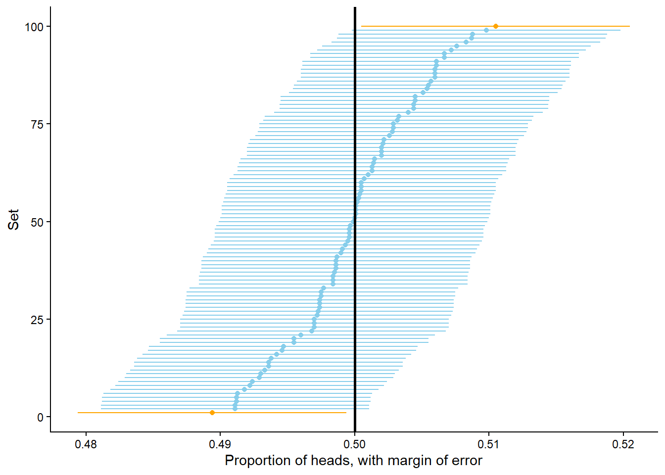
Figure 3.13: Interval estimates of the probability of heads based on 100 sets of **10,000** fair coin flips. Each dot represents the proportion of heads in a set of **10,000** fair coin flips. (The sets have been sorted based on their proportion of heads.) For each set an interval is obtained by adding/subtracting the margin of error of 0.01 from the proportion of heads. In 98 of these 100 sets (the blue dots/intervals) the corresponding interval contains the true probability of heads (0.5, represented by the vertical black line).

What if we want to be stricter about what qualifies as “close to 0.5”? That is, what if a margin of error of 0.01 isn’t good enough? You might suspect that with even more flips we would expect to observe heads on even closer to 50% of flips. Indeed, this is the case. Figure 3.14 displays the results of 100 sets of 1,000,000 fair coin flips. The pattern seems similar to Figure 3.12 but pay close attention to the horizontal axis which covers a much shorter range of values than in the previous figure. Now 91 of the 100 proportions are between 0.499 and 0.501. So in 1,000,000 flips we would expect²⁴ the proportion of heads to be between 0.499 and 0.501, pretty close to 0.5. This suggests that 0.001 might be an appropriate margin of error for a simulation based on 1,000,000 flips.

$data
        phat    ci_lb    ci_ub good_ci
1   0.499578 0.498578 0.500578    TRUE
2   0.500484 0.499484 0.501484    TRUE
3   0.500358 0.499358 0.501358    TRUE
4   0.499911 0.498911 0.500911    TRUE
5   0.498794 0.497794 0.499794   FALSE
6   0.500325 0.499325 0.501325    TRUE
7   0.499705 0.498705 0.500705    TRUE
8   0.499718 0.498718 0.500718    TRUE
9   0.499673 0.498673 0.500673    TRUE
10  0.500370 0.499370 0.501370    TRUE
11  0.499648 0.498648 0.500648    TRUE
12  0.500131 0.499131 0.501131    TRUE
13  0.498816 0.497816 0.499816   FALSE
14  0.500184 0.499184 0.501184    TRUE
15  0.499639 0.498639 0.500639    TRUE
16  0.499542 0.498542 0.500542    TRUE
17  0.499999 0.498999 0.500999    TRUE
18  0.501058 0.500058 0.502058   FALSE
19  0.500083 0.499083 0.501083    TRUE
20  0.500359 0.499359 0.501359    TRUE
21  0.500326 0.499326 0.501326    TRUE
22  0.500136 0.499136 0.501136    TRUE
23  0.499338 0.498338 0.500338    TRUE
24  0.500533 0.499533 0.501533    TRUE
25  0.501039 0.500039 0.502039   FALSE
26  0.500829 0.499829 0.501829    TRUE
27  0.500116 0.499116 0.501116    TRUE
28  0.499673 0.498673 0.500673    TRUE
29  0.499785 0.498785 0.500785    TRUE
30  0.500831 0.499831 0.501831    TRUE
31  0.499648 0.498648 0.500648    TRUE
32  0.500559 0.499559 0.501559    TRUE
33  0.499487 0.498487 0.500487    TRUE
34  0.499637 0.498637 0.500637    TRUE
35  0.499599 0.498599 0.500599    TRUE
36  0.499576 0.498576 0.500576    TRUE
37  0.500547 0.499547 0.501547    TRUE
38  0.501046 0.500046 0.502046   FALSE
39  0.500855 0.499855 0.501855    TRUE
40  0.499686 0.498686 0.500686    TRUE
41  0.500031 0.499031 0.501031    TRUE
42  0.500230 0.499230 0.501230    TRUE
43  0.500837 0.499837 0.501837    TRUE
44  0.500111 0.499111 0.501111    TRUE
45  0.500301 0.499301 0.501301    TRUE
46  0.499950 0.498950 0.500950    TRUE
47  0.499197 0.498197 0.500197    TRUE
48  0.500184 0.499184 0.501184    TRUE
49  0.499879 0.498879 0.500879    TRUE
50  0.500466 0.499466 0.501466    TRUE
51  0.499332 0.498332 0.500332    TRUE
52  0.501171 0.500171 0.502171   FALSE
53  0.499951 0.498951 0.500951    TRUE
54  0.500557 0.499557 0.501557    TRUE
55  0.499955 0.498955 0.500955    TRUE
56  0.499834 0.498834 0.500834    TRUE
57  0.499746 0.498746 0.500746    TRUE
58  0.499565 0.498565 0.500565    TRUE
59  0.500520 0.499520 0.501520    TRUE
60  0.500602 0.499602 0.501602    TRUE
61  0.499545 0.498545 0.500545    TRUE
62  0.500142 0.499142 0.501142    TRUE
63  0.500307 0.499307 0.501307    TRUE
64  0.500380 0.499380 0.501380    TRUE
65  0.499508 0.498508 0.500508    TRUE
66  0.500899 0.499899 0.501899    TRUE
67  0.500220 0.499220 0.501220    TRUE
68  0.498696 0.497696 0.499696   FALSE
69  0.499657 0.498657 0.500657    TRUE
70  0.499487 0.498487 0.500487    TRUE
71  0.499390 0.498390 0.500390    TRUE
72  0.500298 0.499298 0.501298    TRUE
73  0.498958 0.497958 0.499958   FALSE
74  0.499516 0.498516 0.500516    TRUE
75  0.499716 0.498716 0.500716    TRUE
76  0.500268 0.499268 0.501268    TRUE
77  0.499379 0.498379 0.500379    TRUE
78  0.500439 0.499439 0.501439    TRUE
79  0.498707 0.497707 0.499707   FALSE
80  0.500206 0.499206 0.501206    TRUE
81  0.500251 0.499251 0.501251    TRUE
82  0.499538 0.498538 0.500538    TRUE
83  0.500482 0.499482 0.501482    TRUE
84  0.499205 0.498205 0.500205    TRUE
85  0.500057 0.499057 0.501057    TRUE
86  0.499169 0.498169 0.500169    TRUE
87  0.500383 0.499383 0.501383    TRUE
88  0.500239 0.499239 0.501239    TRUE
89  0.499902 0.498902 0.500902    TRUE
90  0.500922 0.499922 0.501922    TRUE
91  0.499574 0.498574 0.500574    TRUE
92  0.500534 0.499534 0.501534    TRUE
93  0.500307 0.499307 0.501307    TRUE
94  0.499403 0.498403 0.500403    TRUE
95  0.499696 0.498696 0.500696    TRUE
96  0.499937 0.498937 0.500937    TRUE
97  0.500142 0.499142 0.501142    TRUE
98  0.499841 0.498841 0.500841    TRUE
99  0.500374 0.499374 0.501374    TRUE
100 0.500431 0.499431 0.501431    TRUE

$layers
$layers[[1]]
geom_dotplot: binaxis = x, stackdir = up, stackratio = 1, dotsize = 1, stackgroups = FALSE, na.rm = FALSE
stat_bindot: binaxis = x, binwidth = NULL, binpositions = bygroup, method = dotdensity, origin = NULL, right = TRUE, width = 0.9, drop = FALSE, na.rm = FALSE
position_identity 

$layers[[2]]
mapping: xintercept = ~xintercept 
geom_vline: na.rm = FALSE
stat_identity: na.rm = FALSE
position_identity 


$scales
<ggproto object: Class ScalesList, gg>
    add: function
    add_defaults: function
    add_missing: function
    backtransform_df: function
    clone: function
    find: function
    get_scales: function
    has_scale: function
    input: function
    map_df: function
    n: function
    non_position_scales: function
    scales: list
    set_palettes: function
    train_df: function
    transform_df: function
    super:  <ggproto object: Class ScalesList, gg>

$guides
<Guides[0] ggproto object>

<empty>

$mapping
$x
<quosure>
expr: ^phat
env:  global

$colour
<quosure>
expr: ^good_ci
env:  global

$fill
<quosure>
expr: ^good_ci
env:  global

attr(,"class")
[1] "uneval"

$theme
$line
$colour
[1] "black"

$linewidth
[1] 0.5

$linetype
[1] 1

$lineend
[1] "butt"

$arrow
[1] FALSE

$inherit.blank
[1] TRUE

attr(,"class")
[1] "element_line" "element"     

$rect
$fill
[1] "white"

$colour
[1] "black"

$linewidth
[1] 0.5

$linetype
[1] 1

$inherit.blank
[1] TRUE

attr(,"class")
[1] "element_rect" "element"     

$text
$family
[1] ""

$face
[1] "plain"

$colour
[1] "black"

$size
[1] 11

$hjust
[1] 0.5

$vjust
[1] 0.5

$angle
[1] 0

$lineheight
[1] 0.9

$margin
[1] 0points 0points 0points 0points

$debug
[1] FALSE

$inherit.blank
[1] TRUE

attr(,"class")
[1] "element_text" "element"     

$title
NULL

$aspect.ratio
NULL

$axis.title
NULL

$axis.title.x
$family
NULL

$face
NULL

$colour
NULL

$size
NULL

$hjust
NULL

$vjust
[1] 1

$angle
NULL

$lineheight
NULL

$margin
[1] 2.75points 0points    0points    0points   

$debug
NULL

$inherit.blank
[1] TRUE

attr(,"class")
[1] "element_text" "element"     

$axis.title.x.top
$family
NULL

$face
NULL

$colour
NULL

$size
NULL

$hjust
NULL

$vjust
[1] 0

$angle
NULL

$lineheight
NULL

$margin
[1] 0points    0points    2.75points 0points   

$debug
NULL

$inherit.blank
[1] TRUE

attr(,"class")
[1] "element_text" "element"     

$axis.title.x.bottom
NULL

$axis.title.y
$family
NULL

$face
NULL

$colour
NULL

$size
NULL

$hjust
NULL

$vjust
[1] 1

$angle
[1] 90

$lineheight
NULL

$margin
[1] 0points    2.75points 0points    0points   

$debug
NULL

$inherit.blank
[1] TRUE

attr(,"class")
[1] "element_text" "element"     

$axis.title.y.left
NULL

$axis.title.y.right
$family
NULL

$face
NULL

$colour
NULL

$size
NULL

$hjust
NULL

$vjust
[1] 1

$angle
[1] -90

$lineheight
NULL

$margin
[1] 0points    0points    0points    2.75points

$debug
NULL

$inherit.blank
[1] TRUE

attr(,"class")
[1] "element_text" "element"     

$axis.text
$family
NULL

$face
NULL

$colour
[1] "grey30"

$size
[1] 0.8 *

$hjust
NULL

$vjust
NULL

$angle
NULL

$lineheight
NULL

$margin
NULL

$debug
NULL

$inherit.blank
[1] TRUE

attr(,"class")
[1] "element_text" "element"     

$axis.text.x
$family
NULL

$face
NULL

$colour
NULL

$size
NULL

$hjust
NULL

$vjust
[1] 1

$angle
NULL

$lineheight
NULL

$margin
[1] 2.2points 0points   0points   0points  

$debug
NULL

$inherit.blank
[1] TRUE

attr(,"class")
[1] "element_text" "element"     

$axis.text.x.top
$family
NULL

$face
NULL

$colour
NULL

$size
NULL

$hjust
NULL

$vjust
[1] 0

$angle
NULL

$lineheight
NULL

$margin
[1] 0points   0points   2.2points 0points  

$debug
NULL

$inherit.blank
[1] TRUE

attr(,"class")
[1] "element_text" "element"     

$axis.text.x.bottom
NULL

$axis.text.y
$family
NULL

$face
NULL

$colour
NULL

$size
NULL

$hjust
[1] 1

$vjust
NULL

$angle
NULL

$lineheight
NULL

$margin
[1] 0points   2.2points 0points   0points  

$debug
NULL

$inherit.blank
[1] TRUE

attr(,"class")
[1] "element_text" "element"     

$axis.text.y.left
NULL

$axis.text.y.right
$family
NULL

$face
NULL

$colour
NULL

$size
NULL

$hjust
[1] 0

$vjust
NULL

$angle
NULL

$lineheight
NULL

$margin
[1] 0points   0points   0points   2.2points

$debug
NULL

$inherit.blank
[1] TRUE

attr(,"class")
[1] "element_text" "element"     

$axis.text.theta
NULL

$axis.text.r
$family
NULL

$face
NULL

$colour
NULL

$size
NULL

$hjust
[1] 0.5

$vjust
NULL

$angle
NULL

$lineheight
NULL

$margin
[1] 0points   2.2points 0points   2.2points

$debug
NULL

$inherit.blank
[1] TRUE

attr(,"class")
[1] "element_text" "element"     

$axis.ticks
$colour
[1] "grey20"

$linewidth
NULL

$linetype
NULL

$lineend
NULL

$arrow
[1] FALSE

$inherit.blank
[1] TRUE

attr(,"class")
[1] "element_line" "element"     

$axis.ticks.x
NULL

$axis.ticks.x.top
NULL

$axis.ticks.x.bottom
NULL

$axis.ticks.y
NULL

$axis.ticks.y.left
NULL

$axis.ticks.y.right
NULL

$axis.ticks.theta
NULL

$axis.ticks.r
NULL

$axis.minor.ticks.x.top
NULL

$axis.minor.ticks.x.bottom
NULL

$axis.minor.ticks.y.left
NULL

$axis.minor.ticks.y.right
NULL

$axis.minor.ticks.theta
NULL

$axis.minor.ticks.r
NULL

$axis.ticks.length
[1] 2.75points

$axis.ticks.length.x
NULL

$axis.ticks.length.x.top
NULL

$axis.ticks.length.x.bottom
NULL

$axis.ticks.length.y
NULL

$axis.ticks.length.y.left
NULL

$axis.ticks.length.y.right
NULL

$axis.ticks.length.theta
NULL

$axis.ticks.length.r
NULL

$axis.minor.ticks.length
[1] 0.75 *

$axis.minor.ticks.length.x
NULL

$axis.minor.ticks.length.x.top
NULL

$axis.minor.ticks.length.x.bottom
NULL

$axis.minor.ticks.length.y
NULL

$axis.minor.ticks.length.y.left
NULL

$axis.minor.ticks.length.y.right
NULL

$axis.minor.ticks.length.theta
NULL

$axis.minor.ticks.length.r
NULL

$axis.line
$colour
[1] "black"

$linewidth
[1] 1 *

$linetype
NULL

$lineend
NULL

$arrow
[1] FALSE

$inherit.blank
[1] FALSE

attr(,"class")
[1] "element_line" "element"     

$axis.line.x
NULL

$axis.line.x.top
NULL

$axis.line.x.bottom
NULL

$axis.line.y
NULL

$axis.line.y.left
NULL

$axis.line.y.right
NULL

$axis.line.theta
NULL

$axis.line.r
NULL

$legend.background
$fill
NULL

$colour
[1] NA

$linewidth
NULL

$linetype
NULL

$inherit.blank
[1] TRUE

attr(,"class")
[1] "element_rect" "element"     

$legend.margin
[1] 5.5points 5.5points 5.5points 5.5points

$legend.spacing
[1] 11points

$legend.spacing.x
NULL

$legend.spacing.y
NULL

$legend.key
NULL

$legend.key.size
[1] 1.2lines

$legend.key.height
NULL

$legend.key.width
NULL

$legend.key.spacing
[1] 5.5points

$legend.key.spacing.x
NULL

$legend.key.spacing.y
NULL

$legend.frame
NULL

$legend.ticks
NULL

$legend.ticks.length
[1] 0.2 *

$legend.axis.line
NULL

$legend.text
$family
NULL

$face
NULL

$colour
NULL

$size
[1] 0.8 *

$hjust
NULL

$vjust
NULL

$angle
NULL

$lineheight
NULL

$margin
NULL

$debug
NULL

$inherit.blank
[1] TRUE

attr(,"class")
[1] "element_text" "element"     

$legend.text.position
NULL

$legend.title
$family
NULL

$face
NULL

$colour
NULL

$size
NULL

$hjust
[1] 0

$vjust
NULL

$angle
NULL

$lineheight
NULL

$margin
NULL

$debug
NULL

$inherit.blank
[1] TRUE

attr(,"class")
[1] "element_text" "element"     

$legend.title.position
NULL

$legend.position
[1] "none"

$legend.position.inside
NULL

$legend.direction
NULL

$legend.byrow
NULL

$legend.justification
[1] "center"

$legend.justification.top
NULL

$legend.justification.bottom
NULL

$legend.justification.left
NULL

$legend.justification.right
NULL

$legend.justification.inside
NULL

$legend.location
NULL

$legend.box
NULL

$legend.box.just
NULL

$legend.box.margin
[1] 0cm 0cm 0cm 0cm

$legend.box.background
list()
attr(,"class")
[1] "element_blank" "element"      

$legend.box.spacing
[1] 11points

$panel.background
$fill
[1] "white"

$colour
[1] NA

$linewidth
NULL

$linetype
NULL

$inherit.blank
[1] TRUE

attr(,"class")
[1] "element_rect" "element"     

$panel.border
list()
attr(,"class")
[1] "element_blank" "element"      

$panel.spacing
[1] 5.5points

$panel.spacing.x
NULL

$panel.spacing.y
NULL

$panel.grid
$colour
[1] "grey92"

$linewidth
NULL

$linetype
NULL

$lineend
NULL

$arrow
[1] FALSE

$inherit.blank
[1] TRUE

attr(,"class")
[1] "element_line" "element"     

$panel.grid.major
list()
attr(,"class")
[1] "element_blank" "element"      

$panel.grid.minor
list()
attr(,"class")
[1] "element_blank" "element"      

$panel.grid.major.x
NULL

$panel.grid.major.y
NULL

$panel.grid.minor.x
NULL

$panel.grid.minor.y
NULL

$panel.ontop
[1] FALSE

$plot.background
$fill
NULL

$colour
[1] "white"

$linewidth
NULL

$linetype
NULL

$inherit.blank
[1] TRUE

attr(,"class")
[1] "element_rect" "element"     

$plot.title
$family
NULL

$face
NULL

$colour
NULL

$size
[1] 1.2 *

$hjust
[1] 0

$vjust
[1] 1

$angle
NULL

$lineheight
NULL

$margin
[1] 0points   0points   5.5points 0points  

$debug
NULL

$inherit.blank
[1] TRUE

attr(,"class")
[1] "element_text" "element"     

$plot.title.position
[1] "panel"

$plot.subtitle
$family
NULL

$face
NULL

$colour
NULL

$size
NULL

$hjust
[1] 0

$vjust
[1] 1

$angle
NULL

$lineheight
NULL

$margin
[1] 0points   0points   5.5points 0points  

$debug
NULL

$inherit.blank
[1] TRUE

attr(,"class")
[1] "element_text" "element"     

$plot.caption
$family
NULL

$face
NULL

$colour
NULL

$size
[1] 0.8 *

$hjust
[1] 1

$vjust
[1] 1

$angle
NULL

$lineheight
NULL

$margin
[1] 5.5points 0points   0points   0points  

$debug
NULL

$inherit.blank
[1] TRUE

attr(,"class")
[1] "element_text" "element"     

$plot.caption.position
[1] "panel"

$plot.tag
$family
NULL

$face
NULL

$colour
NULL

$size
[1] 1.2 *

$hjust
[1] 0.5

$vjust
[1] 0.5

$angle
NULL

$lineheight
NULL

$margin
NULL

$debug
NULL

$inherit.blank
[1] TRUE

attr(,"class")
[1] "element_text" "element"     

$plot.tag.position
[1] "topleft"

$plot.tag.location
NULL

$plot.margin
[1] 5.5points 5.5points 5.5points 5.5points

$strip.background
$fill
[1] "white"

$colour
[1] "black"

$linewidth
[1] 2 *

$linetype
NULL

$inherit.blank
[1] TRUE

attr(,"class")
[1] "element_rect" "element"     

$strip.background.x
NULL

$strip.background.y
NULL

$strip.clip
[1] "inherit"

$strip.placement
[1] "inside"

$strip.text
$family
NULL

$face
NULL

$colour
[1] "grey10"

$size
[1] 0.8 *

$hjust
NULL

$vjust
NULL

$angle
NULL

$lineheight
NULL

$margin
[1] 4.4points 4.4points 4.4points 4.4points

$debug
NULL

$inherit.blank
[1] TRUE

attr(,"class")
[1] "element_text" "element"     

$strip.text.x
NULL

$strip.text.x.bottom
NULL

$strip.text.x.top
NULL

$strip.text.y
$family
NULL

$face
NULL

$colour
NULL

$size
NULL

$hjust
NULL

$vjust
NULL

$angle
[1] -90

$lineheight
NULL

$margin
NULL

$debug
NULL

$inherit.blank
[1] TRUE

attr(,"class")
[1] "element_text" "element"     

$strip.text.y.left
$family
NULL

$face
NULL

$colour
NULL

$size
NULL

$hjust
NULL

$vjust
NULL

$angle
[1] 90

$lineheight
NULL

$margin
NULL

$debug
NULL

$inherit.blank
[1] TRUE

attr(,"class")
[1] "element_text" "element"     

$strip.text.y.right
NULL

$strip.switch.pad.grid
[1] 2.75points

$strip.switch.pad.wrap
[1] 2.75points

attr(,"class")
[1] "theme" "gg"   
attr(,"complete")
[1] TRUE
attr(,"validate")
[1] TRUE

$coordinates
<ggproto object: Class CoordCartesian, Coord, gg>
    aspect: function
    backtransform_range: function
    clip: on
    default: TRUE
    distance: function
    draw_panel: function
    expand: TRUE
    is_free: function
    is_linear: function
    labels: function
    limits: list
    modify_scales: function
    range: function
    render_axis_h: function
    render_axis_v: function
    render_bg: function
    render_fg: function
    reverse: none
    setup_data: function
    setup_layout: function
    setup_panel_guides: function
    setup_panel_params: function
    setup_params: function
    train_panel_guides: function
    transform: function
    super:  <ggproto object: Class CoordCartesian, Coord, gg>

$facet
<ggproto object: Class FacetNull, Facet, gg>
    attach_axes: function
    attach_strips: function
    compute_layout: function
    draw_back: function
    draw_front: function
    draw_labels: function
    draw_panel_content: function
    draw_panels: function
    finish_data: function
    format_strip_labels: function
    init_gtable: function
    init_scales: function
    map_data: function
    params: list
    set_panel_size: function
    setup_data: function
    setup_panel_params: function
    setup_params: function
    shrink: TRUE
    train_scales: function
    vars: function
    super:  <ggproto object: Class FacetNull, Facet, gg>

$plot_env
<environment: R_GlobalEnv>

$layout
<ggproto object: Class Layout, gg>
    coord: NULL
    coord_params: list
    facet: NULL
    facet_params: list
    finish_data: function
    get_scales: function
    layout: NULL
    map_position: function
    panel_params: NULL
    panel_scales_x: NULL
    panel_scales_y: NULL
    render: function
    render_labels: function
    reset_scales: function
    resolve_label: function
    setup: function
    setup_panel_guides: function
    setup_panel_params: function
    train_position: function
    super:  <ggproto object: Class Layout, gg>

$labels
$labels$x
[1] "Proportion of heads"

$labels$colour
[1] "good_ci"

$labels$fill
[1] "good_ci"

$labels$xintercept
[1] "xintercept"

$labels$y
[1] "count"
attr(,"fallback")
[1] TRUE


attr(,"class")
[1] "gg"     "ggplot"

Figure 3.14: Proportion of flips which are heads in 100 sets of 1,000,000 fair coin flips. Each dot represents a set of 1,000,000 fair coin flips. In 91 of these 100 sets the proportion of heads is between 0.499 and 0.501 (the blue dots).

What about even more flips? In Figure 3.15 each dot represents a set of 100 million flips. The pattern seems similar to the previous figures, but again pay close attention the horizontal access which covers a smaller range of values. Now 96 of the 100 proportions are between 0.4999 and 0.5001. So in 100 million flips we would expect²⁵ the proportion of heads to be between 0.4999 and 0.5001, pretty close to 0.5. This suggests that 0.0001 might be an appropriate margin of error for a simulation based on 100,000,000 flips.

$data
         phat     ci_lb     ci_ub good_ci
1   0.4998728 0.4997728 0.4999728   FALSE
2   0.5000130 0.4999130 0.5001130    TRUE
3   0.4999596 0.4998596 0.5000596    TRUE
4   0.4999866 0.4998866 0.5000866    TRUE
5   0.4999105 0.4998105 0.5000105    TRUE
6   0.5001188 0.5000188 0.5002188   FALSE
7   0.5000472 0.4999472 0.5001472    TRUE
8   0.4999685 0.4998685 0.5000684    TRUE
9   0.5000474 0.4999474 0.5001474    TRUE
10  0.5000669 0.4999669 0.5001669    TRUE
11  0.5000429 0.4999429 0.5001429    TRUE
12  0.5000835 0.4999835 0.5001835    TRUE
13  0.4999957 0.4998957 0.5000957    TRUE
14  0.4999895 0.4998895 0.5000895    TRUE
15  0.5000435 0.4999435 0.5001435    TRUE
16  0.4999639 0.4998639 0.5000639    TRUE
17  0.5000452 0.4999453 0.5001452    TRUE
18  0.4999428 0.4998428 0.5000428    TRUE
19  0.4999864 0.4998864 0.5000864    TRUE
20  0.4999838 0.4998838 0.5000838    TRUE
21  0.5000629 0.4999629 0.5001629    TRUE
22  0.5000759 0.4999759 0.5001759    TRUE
23  0.4999714 0.4998714 0.5000714    TRUE
24  0.4999737 0.4998737 0.5000737    TRUE
25  0.5000117 0.4999117 0.5001117    TRUE
26  0.4999804 0.4998804 0.5000804    TRUE
27  0.5000170 0.4999170 0.5001170    TRUE
28  0.5000924 0.4999924 0.5001924    TRUE
29  0.5000129 0.4999129 0.5001129    TRUE
30  0.5000353 0.4999353 0.5001353    TRUE
31  0.5000033 0.4999033 0.5001033    TRUE
32  0.4999509 0.4998509 0.5000509    TRUE
33  0.5000143 0.4999143 0.5001143    TRUE
34  0.5000213 0.4999213 0.5001213    TRUE
35  0.4999975 0.4998975 0.5000975    TRUE
36  0.5000781 0.4999781 0.5001781    TRUE
37  0.5000092 0.4999092 0.5001092    TRUE
38  0.5000498 0.4999498 0.5001498    TRUE
39  0.5000333 0.4999333 0.5001333    TRUE
40  0.5000286 0.4999286 0.5001286    TRUE
41  0.4999952 0.4998952 0.5000952    TRUE
42  0.5000060 0.4999060 0.5001060    TRUE
43  0.4999683 0.4998683 0.5000683    TRUE
44  0.4999649 0.4998649 0.5000649    TRUE
45  0.4999021 0.4998021 0.5000021    TRUE
46  0.5000144 0.4999144 0.5001144    TRUE
47  0.5000737 0.4999737 0.5001737    TRUE
48  0.4999967 0.4998968 0.5000967    TRUE
49  0.5000158 0.4999158 0.5001158    TRUE
50  0.5000015 0.4999015 0.5001015    TRUE
51  0.5000495 0.4999495 0.5001495    TRUE
52  0.5000256 0.4999256 0.5001256    TRUE
53  0.4999712 0.4998712 0.5000712    TRUE
54  0.5000397 0.4999397 0.5001397    TRUE
55  0.5000764 0.4999764 0.5001764    TRUE
56  0.4999523 0.4998523 0.5000523    TRUE
57  0.4999804 0.4998804 0.5000804    TRUE
58  0.4999918 0.4998918 0.5000918    TRUE
59  0.4999884 0.4998884 0.5000884    TRUE
60  0.4999988 0.4998989 0.5000988    TRUE
61  0.4999230 0.4998230 0.5000230    TRUE
62  0.4999605 0.4998605 0.5000605    TRUE
63  0.4999614 0.4998614 0.5000614    TRUE
64  0.5000053 0.4999053 0.5001053    TRUE
65  0.5000153 0.4999153 0.5001153    TRUE
66  0.5000297 0.4999297 0.5001297    TRUE
67  0.4999384 0.4998384 0.5000384    TRUE
68  0.5000174 0.4999174 0.5001174    TRUE
69  0.5000114 0.4999114 0.5001114    TRUE
70  0.4999207 0.4998207 0.5000207    TRUE
71  0.4998804 0.4997804 0.4999804   FALSE
72  0.4999672 0.4998672 0.5000672    TRUE
73  0.4999991 0.4998991 0.5000991    TRUE
74  0.5000081 0.4999081 0.5001081    TRUE
75  0.4999380 0.4998380 0.5000380    TRUE
76  0.5000168 0.4999168 0.5001168    TRUE
77  0.5000849 0.4999849 0.5001849    TRUE
78  0.5000107 0.4999107 0.5001107    TRUE
79  0.5000111 0.4999111 0.5001111    TRUE
80  0.4999935 0.4998935 0.5000935    TRUE
81  0.5000085 0.4999085 0.5001085    TRUE
82  0.4999536 0.4998536 0.5000536    TRUE
83  0.5000203 0.4999203 0.5001203    TRUE
84  0.4999565 0.4998565 0.5000565    TRUE
85  0.4999895 0.4998895 0.5000895    TRUE
86  0.5001008 0.5000008 0.5002008   FALSE
87  0.4999814 0.4998814 0.5000814    TRUE
88  0.4999659 0.4998659 0.5000659    TRUE
89  0.4999704 0.4998704 0.5000704    TRUE
90  0.5000200 0.4999200 0.5001200    TRUE
91  0.5000619 0.4999619 0.5001619    TRUE
92  0.5000026 0.4999026 0.5001026    TRUE
93  0.5000640 0.4999640 0.5001640    TRUE
94  0.4999900 0.4998900 0.5000900    TRUE
95  0.4999018 0.4998018 0.5000018    TRUE
96  0.4999759 0.4998759 0.5000759    TRUE
97  0.5000604 0.4999604 0.5001604    TRUE
98  0.4999934 0.4998934 0.5000934    TRUE
99  0.5000681 0.4999681 0.5001681    TRUE
100 0.4999339 0.4998339 0.5000339    TRUE

$layers
$layers[[1]]
geom_dotplot: binaxis = x, stackdir = up, stackratio = 1, dotsize = 1, stackgroups = FALSE, na.rm = FALSE
stat_bindot: binaxis = x, binwidth = NULL, binpositions = bygroup, method = dotdensity, origin = NULL, right = TRUE, width = 0.9, drop = FALSE, na.rm = FALSE
position_identity 

$layers[[2]]
mapping: xintercept = ~xintercept 
geom_vline: na.rm = FALSE
stat_identity: na.rm = FALSE
position_identity 


$scales
<ggproto object: Class ScalesList, gg>
    add: function
    add_defaults: function
    add_missing: function
    backtransform_df: function
    clone: function
    find: function
    get_scales: function
    has_scale: function
    input: function
    map_df: function
    n: function
    non_position_scales: function
    scales: list
    set_palettes: function
    train_df: function
    transform_df: function
    super:  <ggproto object: Class ScalesList, gg>

$guides
<Guides[0] ggproto object>

<empty>

$mapping
$x
<quosure>
expr: ^phat
env:  global

$colour
<quosure>
expr: ^good_ci
env:  global

$fill
<quosure>
expr: ^good_ci
env:  global

attr(,"class")
[1] "uneval"

$theme
$line
$colour
[1] "black"

$linewidth
[1] 0.5

$linetype
[1] 1

$lineend
[1] "butt"

$arrow
[1] FALSE

$inherit.blank
[1] TRUE

attr(,"class")
[1] "element_line" "element"     

$rect
$fill
[1] "white"

$colour
[1] "black"

$linewidth
[1] 0.5

$linetype
[1] 1

$inherit.blank
[1] TRUE

attr(,"class")
[1] "element_rect" "element"     

$text
$family
[1] ""

$face
[1] "plain"

$colour
[1] "black"

$size
[1] 11

$hjust
[1] 0.5

$vjust
[1] 0.5

$angle
[1] 0

$lineheight
[1] 0.9

$margin
[1] 0points 0points 0points 0points

$debug
[1] FALSE

$inherit.blank
[1] TRUE

attr(,"class")
[1] "element_text" "element"     

$title
NULL

$aspect.ratio
NULL

$axis.title
NULL

$axis.title.x
$family
NULL

$face
NULL

$colour
NULL

$size
NULL

$hjust
NULL

$vjust
[1] 1

$angle
NULL

$lineheight
NULL

$margin
[1] 2.75points 0points    0points    0points   

$debug
NULL

$inherit.blank
[1] TRUE

attr(,"class")
[1] "element_text" "element"     

$axis.title.x.top
$family
NULL

$face
NULL

$colour
NULL

$size
NULL

$hjust
NULL

$vjust
[1] 0

$angle
NULL

$lineheight
NULL

$margin
[1] 0points    0points    2.75points 0points   

$debug
NULL

$inherit.blank
[1] TRUE

attr(,"class")
[1] "element_text" "element"     

$axis.title.x.bottom
NULL

$axis.title.y
$family
NULL

$face
NULL

$colour
NULL

$size
NULL

$hjust
NULL

$vjust
[1] 1

$angle
[1] 90

$lineheight
NULL

$margin
[1] 0points    2.75points 0points    0points   

$debug
NULL

$inherit.blank
[1] TRUE

attr(,"class")
[1] "element_text" "element"     

$axis.title.y.left
NULL

$axis.title.y.right
$family
NULL

$face
NULL

$colour
NULL

$size
NULL

$hjust
NULL

$vjust
[1] 1

$angle
[1] -90

$lineheight
NULL

$margin
[1] 0points    0points    0points    2.75points

$debug
NULL

$inherit.blank
[1] TRUE

attr(,"class")
[1] "element_text" "element"     

$axis.text
$family
NULL

$face
NULL

$colour
[1] "grey30"

$size
[1] 0.8 *

$hjust
NULL

$vjust
NULL

$angle
NULL

$lineheight
NULL

$margin
NULL

$debug
NULL

$inherit.blank
[1] TRUE

attr(,"class")
[1] "element_text" "element"     

$axis.text.x
$family
NULL

$face
NULL

$colour
NULL

$size
NULL

$hjust
NULL

$vjust
[1] 1

$angle
NULL

$lineheight
NULL

$margin
[1] 2.2points 0points   0points   0points  

$debug
NULL

$inherit.blank
[1] TRUE

attr(,"class")
[1] "element_text" "element"     

$axis.text.x.top
$family
NULL

$face
NULL

$colour
NULL

$size
NULL

$hjust
NULL

$vjust
[1] 0

$angle
NULL

$lineheight
NULL

$margin
[1] 0points   0points   2.2points 0points  

$debug
NULL

$inherit.blank
[1] TRUE

attr(,"class")
[1] "element_text" "element"     

$axis.text.x.bottom
NULL

$axis.text.y
$family
NULL

$face
NULL

$colour
NULL

$size
NULL

$hjust
[1] 1

$vjust
NULL

$angle
NULL

$lineheight
NULL

$margin
[1] 0points   2.2points 0points   0points  

$debug
NULL

$inherit.blank
[1] TRUE

attr(,"class")
[1] "element_text" "element"     

$axis.text.y.left
NULL

$axis.text.y.right
$family
NULL

$face
NULL

$colour
NULL

$size
NULL

$hjust
[1] 0

$vjust
NULL

$angle
NULL

$lineheight
NULL

$margin
[1] 0points   0points   0points   2.2points

$debug
NULL

$inherit.blank
[1] TRUE

attr(,"class")
[1] "element_text" "element"     

$axis.text.theta
NULL

$axis.text.r
$family
NULL

$face
NULL

$colour
NULL

$size
NULL

$hjust
[1] 0.5

$vjust
NULL

$angle
NULL

$lineheight
NULL

$margin
[1] 0points   2.2points 0points   2.2points

$debug
NULL

$inherit.blank
[1] TRUE

attr(,"class")
[1] "element_text" "element"     

$axis.ticks
$colour
[1] "grey20"

$linewidth
NULL

$linetype
NULL

$lineend
NULL

$arrow
[1] FALSE

$inherit.blank
[1] TRUE

attr(,"class")
[1] "element_line" "element"     

$axis.ticks.x
NULL

$axis.ticks.x.top
NULL

$axis.ticks.x.bottom
NULL

$axis.ticks.y
NULL

$axis.ticks.y.left
NULL

$axis.ticks.y.right
NULL

$axis.ticks.theta
NULL

$axis.ticks.r
NULL

$axis.minor.ticks.x.top
NULL

$axis.minor.ticks.x.bottom
NULL

$axis.minor.ticks.y.left
NULL

$axis.minor.ticks.y.right
NULL

$axis.minor.ticks.theta
NULL

$axis.minor.ticks.r
NULL

$axis.ticks.length
[1] 2.75points

$axis.ticks.length.x
NULL

$axis.ticks.length.x.top
NULL

$axis.ticks.length.x.bottom
NULL

$axis.ticks.length.y
NULL

$axis.ticks.length.y.left
NULL

$axis.ticks.length.y.right
NULL

$axis.ticks.length.theta
NULL

$axis.ticks.length.r
NULL

$axis.minor.ticks.length
[1] 0.75 *

$axis.minor.ticks.length.x
NULL

$axis.minor.ticks.length.x.top
NULL

$axis.minor.ticks.length.x.bottom
NULL

$axis.minor.ticks.length.y
NULL

$axis.minor.ticks.length.y.left
NULL

$axis.minor.ticks.length.y.right
NULL

$axis.minor.ticks.length.theta
NULL

$axis.minor.ticks.length.r
NULL

$axis.line
$colour
[1] "black"

$linewidth
[1] 1 *

$linetype
NULL

$lineend
NULL

$arrow
[1] FALSE

$inherit.blank
[1] FALSE

attr(,"class")
[1] "element_line" "element"     

$axis.line.x
NULL

$axis.line.x.top
NULL

$axis.line.x.bottom
NULL

$axis.line.y
NULL

$axis.line.y.left
NULL

$axis.line.y.right
NULL

$axis.line.theta
NULL

$axis.line.r
NULL

$legend.background
$fill
NULL

$colour
[1] NA

$linewidth
NULL

$linetype
NULL

$inherit.blank
[1] TRUE

attr(,"class")
[1] "element_rect" "element"     

$legend.margin
[1] 5.5points 5.5points 5.5points 5.5points

$legend.spacing
[1] 11points

$legend.spacing.x
NULL

$legend.spacing.y
NULL

$legend.key
NULL

$legend.key.size
[1] 1.2lines

$legend.key.height
NULL

$legend.key.width
NULL

$legend.key.spacing
[1] 5.5points

$legend.key.spacing.x
NULL

$legend.key.spacing.y
NULL

$legend.frame
NULL

$legend.ticks
NULL

$legend.ticks.length
[1] 0.2 *

$legend.axis.line
NULL

$legend.text
$family
NULL

$face
NULL

$colour
NULL

$size
[1] 0.8 *

$hjust
NULL

$vjust
NULL

$angle
NULL

$lineheight
NULL

$margin
NULL

$debug
NULL

$inherit.blank
[1] TRUE

attr(,"class")
[1] "element_text" "element"     

$legend.text.position
NULL

$legend.title
$family
NULL

$face
NULL

$colour
NULL

$size
NULL

$hjust
[1] 0

$vjust
NULL

$angle
NULL

$lineheight
NULL

$margin
NULL

$debug
NULL

$inherit.blank
[1] TRUE

attr(,"class")
[1] "element_text" "element"     

$legend.title.position
NULL

$legend.position
[1] "none"

$legend.position.inside
NULL

$legend.direction
NULL

$legend.byrow
NULL

$legend.justification
[1] "center"

$legend.justification.top
NULL

$legend.justification.bottom
NULL

$legend.justification.left
NULL

$legend.justification.right
NULL

$legend.justification.inside
NULL

$legend.location
NULL

$legend.box
NULL

$legend.box.just
NULL

$legend.box.margin
[1] 0cm 0cm 0cm 0cm

$legend.box.background
list()
attr(,"class")
[1] "element_blank" "element"      

$legend.box.spacing
[1] 11points

$panel.background
$fill
[1] "white"

$colour
[1] NA

$linewidth
NULL

$linetype
NULL

$inherit.blank
[1] TRUE

attr(,"class")
[1] "element_rect" "element"     

$panel.border
list()
attr(,"class")
[1] "element_blank" "element"      

$panel.spacing
[1] 5.5points

$panel.spacing.x
NULL

$panel.spacing.y
NULL

$panel.grid
$colour
[1] "grey92"

$linewidth
NULL

$linetype
NULL

$lineend
NULL

$arrow
[1] FALSE

$inherit.blank
[1] TRUE

attr(,"class")
[1] "element_line" "element"     

$panel.grid.major
list()
attr(,"class")
[1] "element_blank" "element"      

$panel.grid.minor
list()
attr(,"class")
[1] "element_blank" "element"      

$panel.grid.major.x
NULL

$panel.grid.major.y
NULL

$panel.grid.minor.x
NULL

$panel.grid.minor.y
NULL

$panel.ontop
[1] FALSE

$plot.background
$fill
NULL

$colour
[1] "white"

$linewidth
NULL

$linetype
NULL

$inherit.blank
[1] TRUE

attr(,"class")
[1] "element_rect" "element"     

$plot.title
$family
NULL

$face
NULL

$colour
NULL

$size
[1] 1.2 *

$hjust
[1] 0

$vjust
[1] 1

$angle
NULL

$lineheight
NULL

$margin
[1] 0points   0points   5.5points 0points  

$debug
NULL

$inherit.blank
[1] TRUE

attr(,"class")
[1] "element_text" "element"     

$plot.title.position
[1] "panel"

$plot.subtitle
$family
NULL

$face
NULL

$colour
NULL

$size
NULL

$hjust
[1] 0

$vjust
[1] 1

$angle
NULL

$lineheight
NULL

$margin
[1] 0points   0points   5.5points 0points  

$debug
NULL

$inherit.blank
[1] TRUE

attr(,"class")
[1] "element_text" "element"     

$plot.caption
$family
NULL

$face
NULL

$colour
NULL

$size
[1] 0.8 *

$hjust
[1] 1

$vjust
[1] 1

$angle
NULL

$lineheight
NULL

$margin
[1] 5.5points 0points   0points   0points  

$debug
NULL

$inherit.blank
[1] TRUE

attr(,"class")
[1] "element_text" "element"     

$plot.caption.position
[1] "panel"

$plot.tag
$family
NULL

$face
NULL

$colour
NULL

$size
[1] 1.2 *

$hjust
[1] 0.5

$vjust
[1] 0.5

$angle
NULL

$lineheight
NULL

$margin
NULL

$debug
NULL

$inherit.blank
[1] TRUE

attr(,"class")
[1] "element_text" "element"     

$plot.tag.position
[1] "topleft"

$plot.tag.location
NULL

$plot.margin
[1] 5.5points 5.5points 5.5points 5.5points

$strip.background
$fill
[1] "white"

$colour
[1] "black"

$linewidth
[1] 2 *

$linetype
NULL

$inherit.blank
[1] TRUE

attr(,"class")
[1] "element_rect" "element"     

$strip.background.x
NULL

$strip.background.y
NULL

$strip.clip
[1] "inherit"

$strip.placement
[1] "inside"

$strip.text
$family
NULL

$face
NULL

$colour
[1] "grey10"

$size
[1] 0.8 *

$hjust
NULL

$vjust
NULL

$angle
NULL

$lineheight
NULL

$margin
[1] 4.4points 4.4points 4.4points 4.4points

$debug
NULL

$inherit.blank
[1] TRUE

attr(,"class")
[1] "element_text" "element"     

$strip.text.x
NULL

$strip.text.x.bottom
NULL

$strip.text.x.top
NULL

$strip.text.y
$family
NULL

$face
NULL

$colour
NULL

$size
NULL

$hjust
NULL

$vjust
NULL

$angle
[1] -90

$lineheight
NULL

$margin
NULL

$debug
NULL

$inherit.blank
[1] TRUE

attr(,"class")
[1] "element_text" "element"     

$strip.text.y.left
$family
NULL

$face
NULL

$colour
NULL

$size
NULL

$hjust
NULL

$vjust
NULL

$angle
[1] 90

$lineheight
NULL

$margin
NULL

$debug
NULL

$inherit.blank
[1] TRUE

attr(,"class")
[1] "element_text" "element"     

$strip.text.y.right
NULL

$strip.switch.pad.grid
[1] 2.75points

$strip.switch.pad.wrap
[1] 2.75points

attr(,"class")
[1] "theme" "gg"   
attr(,"complete")
[1] TRUE
attr(,"validate")
[1] TRUE

$coordinates
<ggproto object: Class CoordCartesian, Coord, gg>
    aspect: function
    backtransform_range: function
    clip: on
    default: TRUE
    distance: function
    draw_panel: function
    expand: TRUE
    is_free: function
    is_linear: function
    labels: function
    limits: list
    modify_scales: function
    range: function
    render_axis_h: function
    render_axis_v: function
    render_bg: function
    render_fg: function
    reverse: none
    setup_data: function
    setup_layout: function
    setup_panel_guides: function
    setup_panel_params: function
    setup_params: function
    train_panel_guides: function
    transform: function
    super:  <ggproto object: Class CoordCartesian, Coord, gg>

$facet
<ggproto object: Class FacetNull, Facet, gg>
    attach_axes: function
    attach_strips: function
    compute_layout: function
    draw_back: function
    draw_front: function
    draw_labels: function
    draw_panel_content: function
    draw_panels: function
    finish_data: function
    format_strip_labels: function
    init_gtable: function
    init_scales: function
    map_data: function
    params: list
    set_panel_size: function
    setup_data: function
    setup_panel_params: function
    setup_params: function
    shrink: TRUE
    train_scales: function
    vars: function
    super:  <ggproto object: Class FacetNull, Facet, gg>

$plot_env
<environment: R_GlobalEnv>

$layout
<ggproto object: Class Layout, gg>
    coord: NULL
    coord_params: list
    facet: NULL
    facet_params: list
    finish_data: function
    get_scales: function
    layout: NULL
    map_position: function
    panel_params: NULL
    panel_scales_x: NULL
    panel_scales_y: NULL
    render: function
    render_labels: function
    reset_scales: function
    resolve_label: function
    setup: function
    setup_panel_guides: function
    setup_panel_params: function
    train_position: function
    super:  <ggproto object: Class Layout, gg>

$labels
$labels$x
[1] "Proportion of heads"

$labels$colour
[1] "good_ci"

$labels$fill
[1] "good_ci"

$labels$xintercept
[1] "xintercept"

$labels$y
[1] "count"
attr(,"fallback")
[1] TRUE


attr(,"class")
[1] "gg"     "ggplot"

Figure 3.15: Proportion of flips which are heads in 100 sets of 100,000,000 fair coin flips. Each dot represents a set of 100,000,000 fair coin flips. In 96 of these 100 sets the proportion of heads is between 0.4999 and 0.5001 (the blue dots).

The previous figures illustrate that the more flips there are, the more likely it is that we observe a proportion of flips landing on heads close to 0.5. We also see that with more flips we can refine our definition of “close to 0.5”: increasing the number of flips by a factor of 100 (10,000 to 1,000,000 to 100,000,000) seems to give us an additional decimal place of precision ($0.5\pm0.01$ to $0.5\pm 0.001$ to $0.5\pm 0.0001$.)

3.6.1 A closer look at margin of error

We will now carry out an analysis similar to the one above to investigate simulation margin of error and how it is influenced by the number of simulated values used to compute the relative frequency. Continuing the dice example, suppose we want to estimate $p=\textrm{P}(X=6)$, the probability that the sum of two rolls of a fair four-sided equals six. Since there are 16 possible equally likely outcomes, 3 of which result in a sum of 3, the true probability is $p=3/16=0.1875$.

We will perform a “meta-simulation”. The process is as follows

Simulate two rolls of a fair four-sided die. Compute the sum ($X$) and see if it is equal to 6.
Repeat step 1 to generate $N$ simulated values of the sum ($X$). Compute the relative frequency of sixes: count the number of the $N$ simulated values equal to 6 and divide by $N$. Denote this relative frequency $\hat{p}$ (read “p-hat”).
Repeat step 2 a large number of times, recording the relative frequency $\hat{p}$ for each set of $N$ values.

Be sure to distinguish between steps 2 and 3. A simulation will typically involve just steps 1 and 2, resulting in a single relative frequency based on $N$ simulated values. Step 3 is the “meta” step; we see how this relative frequency varies from simulation to simulation to help us in determing an appropriate margin of error. The important quantity in this analysis is $N$, the number of independently simulated values used to compute the relative frequency in a single simulation. We wish to see how $N$ impacts margin of error. The number of simulations in step 3 just needs to be “large” enough to provide a clear picture of how the relative frequency varies from simulation to simulation. The more the relative frequency varies from simulation to simulation, the larger the margin of error needs to be.

We can combine steps 1 and 2 of the meta-simulation to put it in the framework of the simulations from earlier in this chapter. Namely, we can code the meta-simulation as a single simulation in which

A sample space outcome represents $N$ values of the sum of two fair-four sided dice
The main random variable of interest is the proportion of the $N$ values which are equal to 6.

Let’s first consider $N=100$. The following Symbulate code defines the probability space corresponding to 100 values of the sum of two-fair four sided dice. Notice the use of apply which functions much in the same way²⁶ as RV.

N = 100
P = BoxModel([1, 2, 3, 4], size = 2).apply(sum) ** N
P.sim(5)

Index	Result
0	(5, 6, 6, 4, 5, ..., 8)
1	(7, 4, 4, 3, 7, ..., 5)
2	(8, 3, 6, 4, 5, ..., 4)
3	(8, 5, 6, 7, 6, ..., 7)
4	(2, 5, 5, 7, 6, ..., 4)

In the code above

BoxModel([1, 2, 3, 4], size = 2) simulates two rolls of a fair four-sided die
.apply(sum) computes the sum of the two rolls
** N repeats the process N times to generate a set of N independent values, each value representing the sum of two rolls of a fair four-sided die
P.sim(5) simulates 5 sets, each set consisting of N sums

Now we define the random variable which takes as an input a set of $N$ sums and returns the proportion of the $N$ sums which are equal to six.

phat = RV(P, count_eq(6)) / N
phat.sim(5)

Index	Result
0	0.19
1	0.17
2	0.15
3	0.17
4	0.19

In the code above

phat is an RV defined on the probability space P. Recall that an outcome of P is a set of N sums (and each sum is the sum of two rolls of a fair four-sided die).
The function that defines the RV is count.eq(6), which counts the number of values in the set that are equal to 6. We then²⁷ divide by N, the total number of values in the set, to get the relative frequency. (Remember that a transformation of a random variable is also a random variable.)
phat.sim(5) generates 5 simulated values of the relative frequency phat. Each simulated value of phat is the relative frequency of sixes in N sums of two rolls of a fair four-sided die.

Now we simulate and summarize a large number of values of phat. We’ll simulate 100 values for illustration (as we did in Figure 3.12, Figure 3.14, and Figure 3.15). Be sure not to confuse 100 with N. Remember, the important quantity is N, the number of simulated values used in computing each relative frequency.

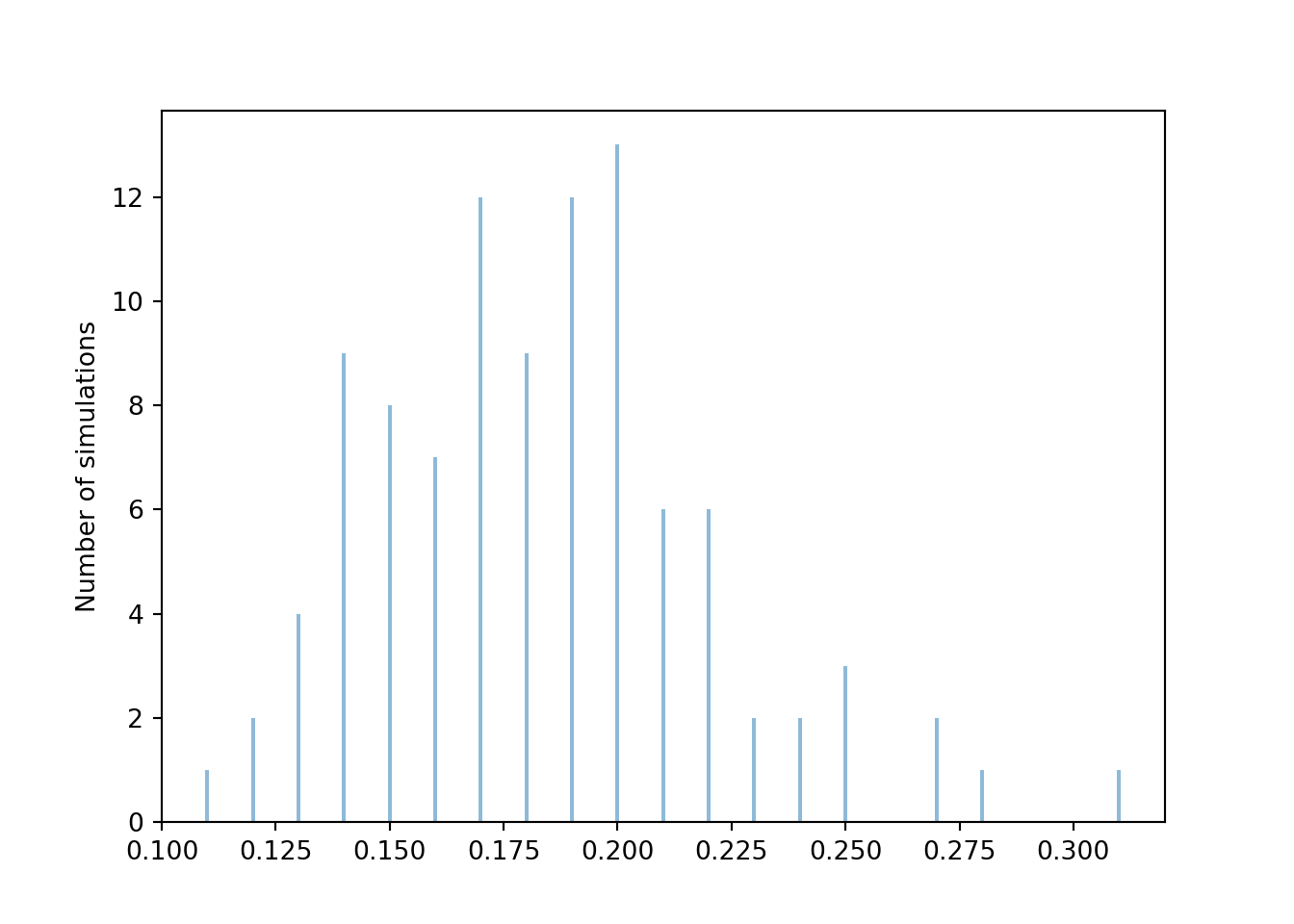
phat.sim(100).plot(type = "impulse", normalize = False)
plt.ylabel('Number of simulations');

We see that the 100 relative frequencies are roughly centered around the true probability 0.1875, but there is variability in the relative frequencies from simulation to simulation. From the range of values, we see that most relative frequencies are within about 0.08 or so from the true probability 0.1875. So a value around 0.08 seems like a reasonable value of the margin of error, but the actual value depends on what we mean by “most”. We can get a clearer picture if we run more simulations. The following plot displays the results of 10000 simulations, each resulting in a value of $\hat{p}$. Remember that each relative frequency is based on $N=100$ sums of two rolls.

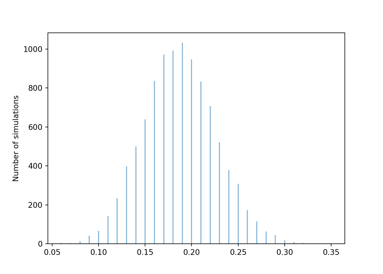
phats = phat.sim(10000)
phats.plot(type = "impulse", normalize = False)
plt.ylabel('Number of simulations');

Let’s see how many of these 10000 simulated proportions are within 0.08 of the true probability 0.1875.

1 - (phats.count_lt(0.1875 - 0.08) + phats.count_gt(0.1875 + 0.08)) / 10000

0.9609

In roughly 95% or so of simulations, the simulated relative frequency was within 0.08 of the true probability. So 0.08 seems like a reasonable margin of error for “95% confidence” or “95% accuracy”. However, a margin of error of 0.08 yields pretty imprecise estimates, ranging from about 0.10 to 0.27. Can we keep the degree of accuracy at 95% but get a smaller margin of error, and hence a more precise estimate? Yes, if we increase the number of repetitions used to compute the relative frequency.

Now we repeat the analysis, but with $N=10000$. In this case, each relative frequency is computed based on 10000 independent values, each value representing a sum of two rolls of a fair four-sided die. As before we start with 100 simulated relative frequencies.

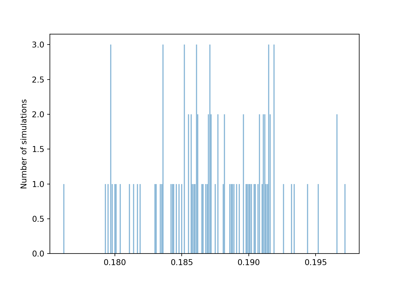
N = 10000
P = BoxModel([1, 2, 3, 4], size = 2).apply(sum) ** N
phat = RV(P, count_eq(6)) / N

phats = phat.sim(100)
phats.plot(type = "impulse", normalize = False)
plt.ylabel('Number of simulations');

Again we see that the 100 relative frequencies are roughly centered around the true probability 0.1875, but there is less variability in the relative frequencies from simulation to simulation for $N=10000$ than for $N=100$. Pay close attention to the horizontal axis. From the range of values, we see that most relative frequencies are now within about 0.008 of the true probability 0.1875.

1 - (phats.count_lt(0.1875 - 0.008) + phats.count_gt(0.1875 + 0.008)) / 100

0.95

As with $N=100$, running more than 100 simulations would give a clearer picture of how much the relative frequency based on $N=10000$ simulated values varies from simulation to simulation. But even with just 100 simulations, we see that a margin of error of about 0.008 is required for roughly 95% accuracy when $N=10000$, as opposed to 0.08 when $N=100$. As we observed in the coin flipping example earlier in this section, it appears that increasing $N$ by a factor of 100 yields an extra decimal place of precision. That is, increasing $N$ by a factor of 100 decreases the margin of error by a factor of $\sqrt{100}$. In general, the margin of error is inversely related to $\sqrt{N}$.

Table 3.9: Comparison of margins of error for 95% confidence for the meta-simulations in this section.

Probability that	True value	95% m.o.e. (N = 100)	95% m.o.e. (N = 10000)	95% m.o.e. (N = 1000000)
A fair coin flip lands H	0.5000	0.1000	0.0100	0.0010
Two rolls of a fair four-sided die sum to 6	0.1875	0.0781	0.0078	0.0008

The two examples in this section illustrate that the margin of error also depends somewhat on the true probability. The margin of error required for 95% accuracy is larger when the true probability is 0.5 than when it is 0.1875. It can be shown that when estimating a probability $p$ with a relative frequency based on $N$ simulated repetitions, the margin of error required for 95% confidence²⁸ is \[ 2\frac{\sqrt{p(1-p)}}{\sqrt{N}} \] For a given $N$, the above quantity is maximized when $p$ is 0.5. Since $p$ is usually unknown—the reason for performing the simulation is to approximate it—we plug in 0.5 for a somewhat conservative margin of error of $1/\sqrt{N}$.

For a fixed $N$, there is a tradeoff between accuracy and precision. The factor 2 in the margin of error formula above corresponds to 95% accuracy. Greater accuracy would require a larger factor, and a larger margin of error, resulting in a wider—that is, less precise—interval. For example, 99% confidence requires a factor of roughly 2.6 instead of 2, resulting in an interval that is roughly 30 percent wider. The confidence level does matter, but the primary influencer of margin of error is $N$, the number of independently simulated repetitions on which the relative frequency is based. Regardless of confidence level, the margin of error is on the order of magnitude of $1/\sqrt{N}$.

In summary, the margin of error when approximating a probability based on a simulated relative frequency is roughly on the order $1/\sqrt{N}$, where $N$ is the number of independently simulated repetitions used to calculate the relative frequency. Warning: alternative methods are necessary when the actual probability being estimated is very close to 0 or to 1.

A probability is a theoretical long run relative frequency. A probability can be approximated by a relative frequency from a large number of simulated repetitions, but there is some simulation margin of error. Likewise, the average value of $X$ after a large number of simulated repetitions is only an approximation to the theoretical long run average value of $X$, that is, the expected value of $X$. The margin of error is also on the order of $1/\sqrt{N}$ where $N$ is the number of independently simulated values used to compute the average, but the degree of variability of the random variable also plays a role. We will explore margins of error for long run averages in more detail later.

Pay attention to what $N$ denotes: $N$ is the number of independently²⁹ simulated repetitions used to calculate the relative frequency. This is not necessarily the number of simulated repetitions. For example, suppose we use simulation to approximate the conditional probability that the larger of two rolls of a fair four-sided die is 4 given that the sum is equal to 6. We might start by simulating 10000 pairs of rolls. But the sum would be equal to 6 in only about 1875 pairs, and it is only these pairs that would be used to compute the relative frequency that the larger roll is 4 to approximate the probability of interest. The appropriate margin of error is roughly $1/\sqrt{1875} \approx 0.023$. Compared to 0.01 (based on the original 10000 repetitions), the margin of error of 0.023 for the conditional probability results in intervals that are 130 percent wider. Carefully identifying the number of repetitions used to calculate the relative frequency is especially important when determining appropriate simulation margins of error for approximating conditional probabilities, which we’ll discuss in more detail later.

3.6.2 Approximating multiple probabilities

When using simulation to estimate a single probability, the primary influencer of margin of error is $N$, the number of repetitions on which the relative frequency is based. It doesn’t matter as much whether we use, say, 95% versus 99% confidence (either way, it’s an “A”). That is, it doesn’t matter too much whether we compute our margin of error using \[ 2\frac{\sqrt{p(1-p)}}{\sqrt{N}}, \] with a multiple of 2 for 95% confidence, or if we replace 2 by 2.6 for 99% confidence. (Remember, we can plug in 0.5 for the unknown $p$ for a conservative margin of error.) A margin of error based on 95% or 99% (or another confidence level in the neighborhood) provides a reasonably accurate estimate of the probability. However, using simulation to approximate multiple probabilities simultaneously requires a little more care with the confidence level.

In the previous section we used simulation to estimate $\textrm{P}(X=6)$. Now suppose we want to approximate $\textrm{P}(X = x)$ for each value of $x = 2,3,4,5,6,7,8$. We could run a simulation to obtain results like those in Figure 3.11 and the table before it. Each of the relative frequencies in the table is an approximation of the true probability, and so each of the relative frequencies should have a margin of error, say 0.01 for a simulation based on 10000 repetitions. Thus, the simulation results yield a collection of seven interval estimates, an interval estimate of $\textrm{P}(X = x)$ for each value of $x = 2,3,4,5,6,7,8$. Each interval in the collection either contains the respective true probability or not. The question is then: In what percent of simulations will every interval in the collection contain the respective true probability?

Figure 3.16 summarizes the results of 100 simulations. Each simulation consists of 10000 repetitions, with results similar to those in Figure 3.11 and the table before it. Each simulation is represented by a row in Figure 3.16, consisting of seven 95% interval estimates, one for each value of $x$. (The rows have been sorted before plotting; see the next paragraph.) Each panel represents a different value of $x$; for each value of $x$, around 95 out of the 100 simulations yield estimates that contain the true probability $\textrm{P}(X=x)$, represented by the vertical line.

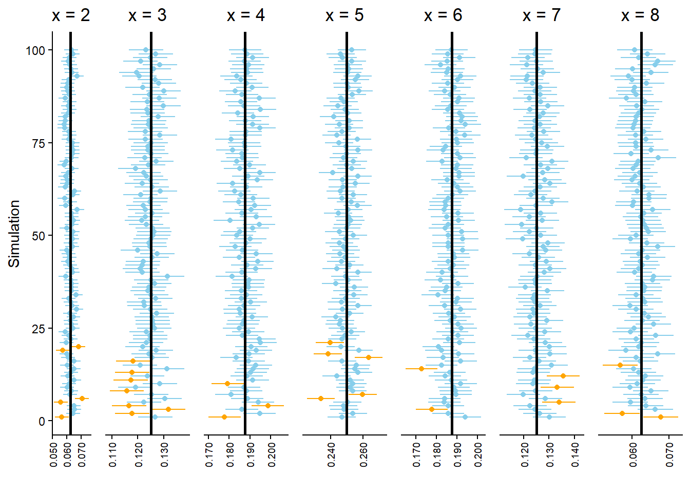
Figure 3.16: Results of 100 simulations. Each simulation yields a collection of seven 95% confidence intervals.

However, let’s zoom in on the bottom of Figure 3.16. Figure 3.17 displays the results of the 21 simulations at the bottom of Figure 3.16. Look carefully row by row in Figure 3.17; in each of these simulations at least one of the seven intervals in the collection does not contain the true probability. In other words, every interval in the collection contains the respective true probability in only 79 of the 100 simulations (the other simulations in Figure 3.16).) While we have 95 percent confidence in our interval estimate of $\textrm{P}(X = x)$ for any single $x$, we only have around 79 percent confidence in our approximate distribution of $X$. Our confidence “grade” has gone from “A” range (95 percent) to “C” range (79 percent).

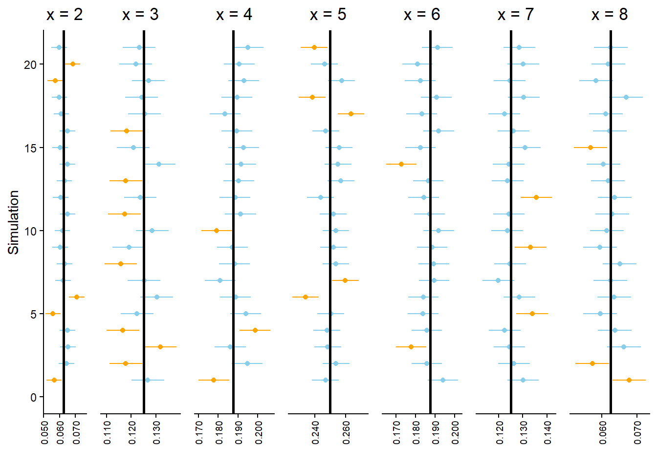
Figure 3.17: Subset of 21 simulations from Figure 3.16. In each of these simulations, at least one 95% confidence interval does not contain the respective true probability.

When approximating multiple probabilities based on a single simulation, such as when approximating a distribution, margins of error and interval estimates need to be adjusted to obtain simultaneous 95% confidence. The easiest way to do this is to make all of the intervals in the collection wider.

There are many procedures for adjusting a collection of interval estimates to achieve simultaneous confidence; we won’t get into any technical details. As a very rough, but simple and typically conservative rule, when approximating many probabilities based on a single simulation, we recommend making the margin of error twice as large as when approximating a single probability. That is, use a margin of error of $2/\sqrt{N}$ (rather than $1/\sqrt{N}$) to achieve simultaneous 95% confidence when approximating many probabilities based on a single simulation.

Figure 3.18 displays the same simulation results as Figure 3.16, but now the margin of error for each confidence interval is 2 times greater. We can see that all of the original “bad” intervals turn “good” when widened, and now there is (greater than) 95% simultaneous confidence.

Figure 3.18: Results of 100 simulations. Each simulation yields a collection of seven 95% confidence intervals. The margin of error has been adjusted to obtain simultaneous confidence.

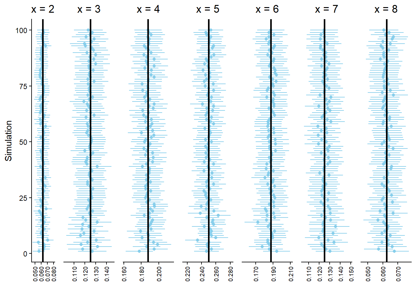
3.6.3 Beware a false sense of precision

Why don’t we always run something like one trillion repetitions so that our margin of error is tiny? There is a cost to simulating and storing more repetitions in terms of computational time and memory. Also, remember that simulating one trillion repetitions doesn’t guarantee that the margin of error is actually based on anywhere close to one trillion repetitions, especially when conditioning on a low probability event.

Most importantly, keep in mind that any probability model is based on a series of assumptions and these assumptions are not satisfied exactly by the random phenomenon. A precise estimate of a probability under the assumptions of the model is not necessarily a comparably precise estimate of the true probability. Reporting probability estimates out to many decimal places conveys a false sense of precision and should typically be avoided.

For example, the probability that any particular coin lands on heads is probably not 0.5 exactly. But any difference between the true probability of the coin landing on heads and 0.5 is likely not large enough to be practically meaningful³⁰. That is, assuming the coin is fair is a reasonable model.

Suppose we assume that the probability that a coin lands on heads is exactly 0.5 and that the results of different flips are independent. If we flip the coin 1000 times the probability that it lands on heads at most 490 times is 0.2739864. (We will see a formula for computing this value later.) If we were to simulate one trillion repetitions (each consisting of 1000 flips) to estimate this probability then our margin of error would be 0.000001; we could expect accuracy out to the sixth decimal place. However, reporting the probability with so many decimal places is somewhat disingenuous. If the probability that the coin lands on heads were 0.50001, then the probability of at most 490 heads in 1000 flips would be 0.2737757. If the probability that the coin lands on heads were 0.5001, then the probability of at most 490 heads in 1000 flips would be 0.2718834. Reporting our approximate probability as something like 0.2739864 $\pm$ 0.000001 says more about the precision in our assumption that the coin is fair than it does about the true probability that the coin lands on heads at most 490 times in 1000 flips. A more honest conclusion would result from running 10000 repetitions and reporting our approximate probability as something like 0.27 $\pm$ 0.01. Such a conclusion reflects more genuinely that there’s some “wiggle room” in our assumptions, and that any probability computed according to our model is at best a reasonable approximation of the “true” probability.

For most of the situations we’ll encounter in this book, estimating a probability to within 0.01 of its true value will be sufficient for practical purposes, and so basing approximations on 10000 independently simulated values will be appropriate. Of course, there are real situations where probabilities need to be estimated much more precisely, e.g., the probability that a bridge will collapse. Such situations require more intensive methods.

Example 3.9 Donny Dont runs a simulation to approximate the probability of an event $A$. In 1,000,000 repetitions, event $A$ occurs on 437,952 repetitions. He computes a margin of error (for 95% confidence) of $1/\sqrt{1000000} = 0.001$. Donny tries a few different ways of reporting his results. Explain to him what is wrong, missing, or could be improved in each of the following.

I estimate that $\textrm{P}(A)$ is 0.437952.
I estimate that $\textrm{P}(A)$ is 43.7952% with a margin of error of 0.1%.
I estimate that $\textrm{P}(A)$ is between 0.436952 and 0.438952.
I estimate with 95% confidence that under these assumptions $\textrm{P}(A)$ is between 0.437 and 0.439.

Solution (click to expand)

Solution 3.9.

Donny has not provided a margin of error.
We’re okay with Donny expressing the proportion as a percent. However, 0.001 is technically a margin of error of 0.1 percentage points. A margin of error of 0.1% implies a percentage change, leading to interval endpoints of $0.437952\times (1 - 0.001) = 0.437514$ and $0.437952\times (1 + 0.001) = 0.438390$. With a margin of error of 0.001, the interval endpoints are really $0.437952 - 0.001 = 0.436952$ and $0.437952 + 0.001 = 0.438952$. The numbers are fairly similar in this case, but in general, the margins of error we have discussed are additive and therefore should be reported as percentage points.
We don’t know the context, but in many situations reporting estimates to six decimal places as Donny has done is not necessary and could convey a false sense of precision.
We like Donny’s statement! He has provided an interval estimate, reported his level of confidence, rounded to an appropriate number of decimal places (in most contexts) so as not to convey a false sense of precision, and drawn attention to to the fact that the estimate of the probability is predicated on the model assumptions. It would have also been fine if he had replaced “is between 0.437 and 0.439” with “is 0.438 with a margin of error of 0.001”. In practice, Donny should replace vague statements like “these assumptions” and “$\textrm{P}(A)$” with contextual details, but the general form of his answer is very good.

3.6.4 Exercises

Exercise 3.16 Use simulation to approximate the probability that at least two people in a group of $n=30$ share a birthday in Example 2.48. Compute the margin of error and write a clearly worded sentence reporting your approximate probability in context.

Exercise 3.17 The latest series of collectible Lego Minifigures contains 3 different Minifigure prizes (labeled 1, 2, 3). Each package contains a single unknown prize. Suppose we only buy 3 packages and we consider as our sample space outcome the results of just these 3 packages (prize in package 1, prize in package 2, prize in package 3). For example, 323 (or (3, 2, 3)) represents prize 3 in the first package, prize 2 in the second package, prize 3 in the third package. Let $X$ be the number of distinct prizes obtained in these 3 packages. Let $Y$ be the number of these 3 packages that contain prize 1.

Suppose you simulate 10000 $(X, Y)$ pairs and use the results to approximate all of

Marginal distribution of $X$
Marginal distribution of $Y$
Joint distribution of $X$ and $Y$

What is the approximate margin of error for simultaneous 95% confidence?

3.7 Approximating expected values: Averages

On any single repetition of a simulation a particular event either occurs or not. Summarizing simulation results for events involves simply counting the number of repetitions on which the event occurs and finding related proportions.

On the other hand, random variables typically take many possible values over the course of many repetitions. We are still interested in relative frequencies of events, like $\{X=6\}$, $\{Y \ge 3\}$, and $\{X > 5, Y \ge 3\}$. But for random variables we are also interested in their distributions which describe the possible values that the random variables can take and their relative likelihoods. A marginal distribution contains all the information about the pattern of variability of a single random variable alone, and a joint distribution contains all the information about the pattern of variability of a collection of random variables. It is also useful to summarize some key features of the pattern of variability.

One summary characteristic of a marginal distribution of a random variable is the expected value. In Section 1.7 and Section 2.5.3 we discussed how an expected value can be interpreted as the long run average value of a random variable. We can approximate the long run average value by simulating many values of the random variable and computing the average (a.k.a. mean) in the usual way: sum all the simulated values and divide by the number of simulated values.

Example 3.10 Let $X$ be the sum of two rolls of a fair four-sided die, and let $Y$ be the larger of the two rolls (or the common value if a tie). Recall your tactile simulation from Example 3.1; see ours in Table 3.1. Based only on the results of your simulation, approximate the long run average value of each of the following. (Don’t worry if the approximations are any good yet.)

$X$
$Y$
$X^2$
$XY$

Solution (click to expand)

Solution 3.10. We reproduce the results of our simulation in Table 3.10 with additional columns for $X^2$ and $XY$. Results vary naturally so your simulation results will be different, but the same ideas apply.

Table 3.10: Results of 10 repetitions of two rolls of a fair four-sided die

Results of 10 repetitions of two rolls of a fair four-sided die
Repetition	First roll	Second roll	X	Y	X^2	XY
1	2	1	3	2	9	6
2	1	1	2	1	4	2
3	3	3	6	3	36	18
4	4	3	7	4	49	28
5	3	2	5	3	25	15
6	3	4	7	4	49	28
7	2	3	5	3	25	15
8	2	4	6	4	36	24
9	1	2	3	2	9	6
10	3	4	7	4	49	28

Approximate the long run average value of $X$ by summing the 10 simulated values of $X$ and dividing by 10. \[ \frac{3 + 2 + 6 + 7 + 5 + 7 + 5 + 6 + 3 + 7}{10} = 5.1 \]
Approximate the long run average value of $Y$ by summing the 10 simulated values of $Y$ and dividing by 10. \[ \frac{2 + 1 + 3 + 4 + 3 + 4 + 3 + 4 + 2 + 4}{10} = 3 \]
First, for each repetition square the value of $X$ to obtain the $X^2$ column. Then approximate the long run average value of $X^2$ by summing the 10 simulated values of $X^2$ and dividing by 10. \[ \frac{9 + 4 + 36 + 49 + 25 + 49 + 25 + 36 + 9 + 49}{10} = 29.1 \]
First, for each repetition compute the product $XY$ to obtain the $XY$ column. Then approximate the long run average value of $XY$ by summing the 10 simulated values of $XY$ and dividing by 10. \[ \frac{6 + 2 + 18 + 28 + 15 + 28 + 15 + 24 + 6 + 28}{10} = 17 \]

Of course, 10 repetitions is not enough to reliably approximate the long run average value. But whether the average is based on 10 values or 10 million, an average is computed in the usual way: sum the values and divide by the number of values.

Example 3.11 Recall Section 3.2.2 where we assumed the arrival time $X$ (minutes after noon) followed a Normal(30, 10) distribution, represented by the spinner in Figure 3.7. Table 3.5 displays 10 simulated values of $X$. Based only on the results of this simulation, approximate the long run average value of $X$. (Don’t worry if the approximation is any good yet.)

Solution (click to expand)

Solution 3.11. Approximate the long run average value of $X$ by simply computing the average in the usual way: sum the 10 simulated values of $X$ and divide by 10. It’s just that when $X$ is continuous each simulated value will be distinct with lots of decimal places.

\[ {\scriptscriptstyle \frac{21.387... + 50.719... + 24.09... + 32.68... + 54.511... + 38.117... + 16.819... + 22.98... + 28.867... + 43.43}{10} = 33.36 } \]

We have seen a few examples of how to compute expected values for discrete random variables as probability-weighted average values. The computation of expected values for continuous random variables is more complicated. However, expected values can also be interpreted as long run average values for continuous random variables. Therefore, expected values can be approximated in the same way for discrete and continuous random variables: simulate lots of values and compute the average.

In the examples in the section we only considered 10 simulated repetitions to emphasize that we’re simply computing an average in the usual way. But to get a good approximation of an expected value, we’ll need to simulate many more values and average. We’ll soon explore what happens to the average as we simulate more values, but first a caution about averages of transformations.

3.7.1 Averages of transformations

Example 3.12 Donny Don’t says: “In Example 3.10, why bother creating columns for $X^2$ and $XY$? If I want to find the average value of $X^2$ I can just square the average value of $X$. For the average value of $XY$ I can just multiply the average value of $X$ and the average value of $Y$.” Do you agree? (Check to see if this works for your simulation results.) If not, explain why not.

Solution (click to expand)

Solution 3.12. It is easy to check that Donny has made a mistake just by inspecting the simulation results: 5.1² $\neq$ 29.1, 5.1 $\times$ 3 $\neq$ 17. To see why, suppose we had just performed two repetitions, resulting in the first two rows of Table 3.10.

\[ \text{Average of $X^2$} = \frac{3^2 + 2^2}{2} =6.5 \neq 6.25= \left(\frac{3 + 2}{2}\right)^2=(\text{Average of $X$})^2 \]

Squaring first and then averaging (which yields 6.5) is not the same as averaging first and then squaring (which yields 6.25), essentially because $(3+2)^2\neq 3^2 + 2^2$.

Similarly, \[ {\small \text{Average of $XY$} = \frac{(3)(2) + (2)(1)}{2} =4 \neq 3.75= \left(\frac{3 + 2}{2}\right)\left(\frac{2 + 1}{2}\right)=(\text{Average of $X$})\times (\text{Average of $Y$}) } \] Multiplying first and then averaging (which yields 4) is not the same as averaging first and then multiplying (which yields 3.75), essentially because $(3)(2)+(2)(1)\neq(3+2)(2+1)$.

We often transform random variables to obtain other random variables, e.g. $X$ to $g(X)$. To obtain the average of the transformed variable, we cannot simply plug the average of the original variable into the transformation formula. Instead, we need to transform the values of the variable first and then average the transformed values. In general the order of transforming and averaging is not interchangeable. Whether in the short run or the long run, in general \[\begin{align*} \text{Average of $g(X)$} & \neq g(\text{Average of $X$})\\ \text{Average of $g(X, Y)$} & \neq g(\text{Average of $X$}, \text{Average of $Y$}) \end{align*}\]

In terms of expected value, in general \[\begin{align*} \textrm{E}(g(X)) & \neq g(\textrm{E}(X))\\ \textrm{E}(g(X, Y)) & \neq g(\textrm{E}(X), \textrm{E}(Y)) \end{align*}\]

Warning

Be careful! Many common mistakes in probability result from not heeding this general principle about averages (expected values) of transformations.

3.7.2 Long run averages

We have investigated long run relative frequencies; see Section 1.2.1 and Section 3.6 in particular. Now let’s see what happens to averages in the long run. Continuing Example 3.10 let $X$ be the sum of two rolls of a fair four-sided die. Table 3.11 displays the results of 10 pairs of rolls of a fair four-sided die. The first column is the repetition number (first pair, second pair, and so on) and the second column represents $X$, the sum of the two rolls. The third column displays the running sum of $X$ values, and the fourth column the running average of $X$ values. Figure 3.19 displays the running average as a function of the number of repetitions. Of course, the results depend on the particular sequence of rolls. We encourage you to roll the dice and construct your own table and plot.

Table 3.11: Results and running average of $X$, the sum of two rolls of a fair four-sided die.

Repetition	Value of X	Running sum of X	Running average of X
1	3	3	3.000
2	2	5	2.500
3	6	11	3.667
4	7	18	4.500
5	5	23	4.600
6	7	30	5.000
7	5	35	5.000
8	6	41	5.125
9	3	44	4.889
10	7	51	5.100

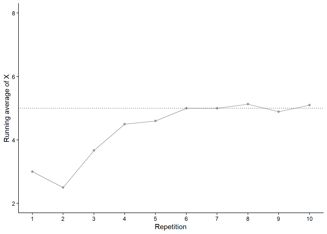
Figure 3.19: Running average of $X$ for the 10 pairs of rolls in Table 3.11.

Now we’ll perform 90 more repetitions for a total of 100. Figure 3.20 (a) summarizes the results, while Figure 3.20 (b) also displays the results for 3 additional simulations of 100 pairs of rolls. The running average fluctuates considerably in the early stages, but settles down and tends to get closer to 5 as the number of repetitions increases. However, each of the four simulations results in a different average of $X$ after 100 pairs of rolls: 4.85 (gray), 4.9 (orange), 5.25 (blue), 4.79 (green). Even after 100 pairs of rolls the running average of $X$ still fluctuates from simulation to simulation.

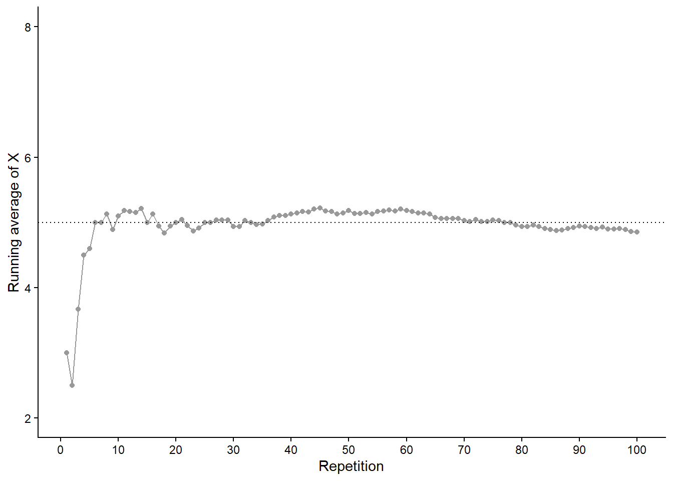
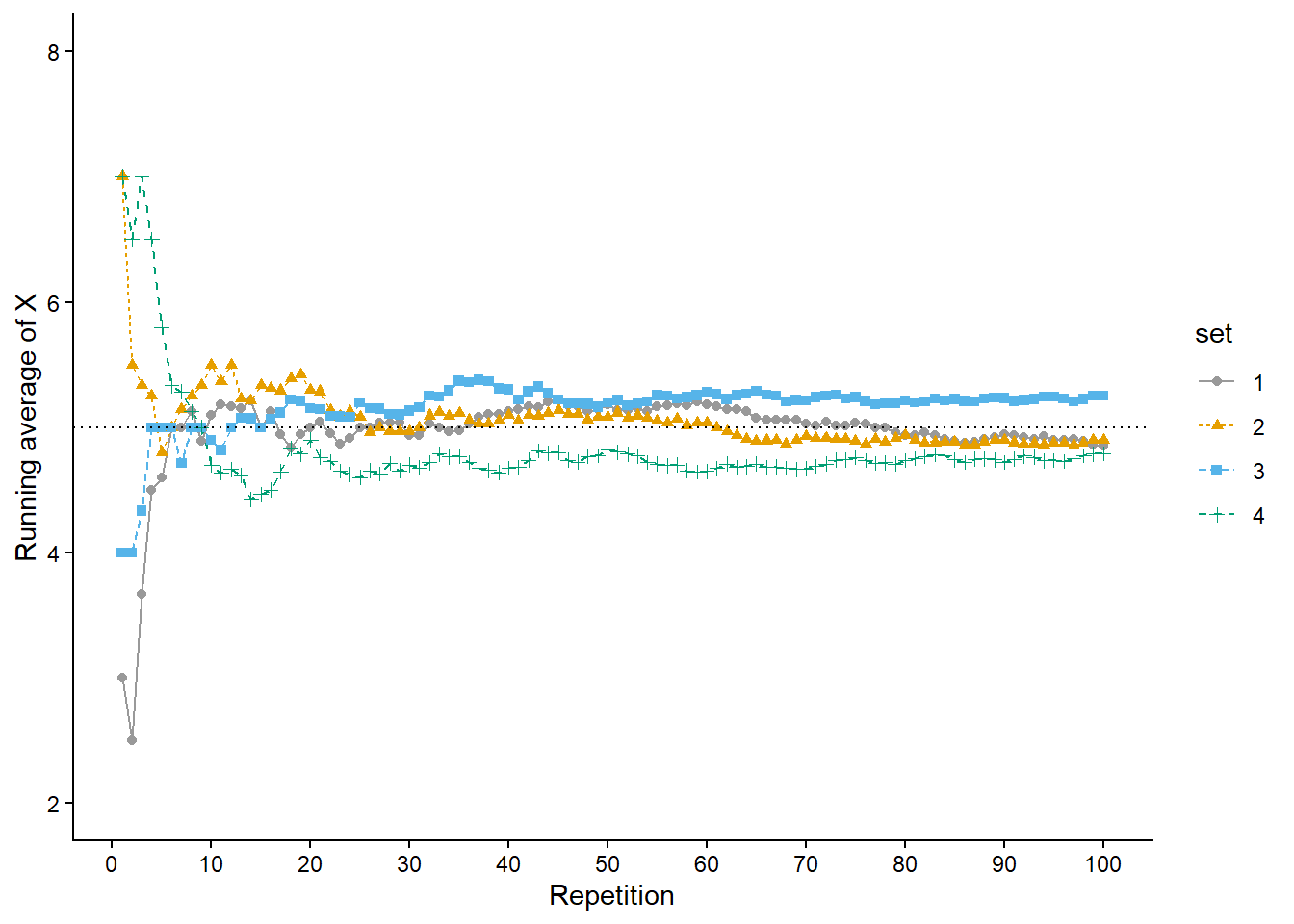
(a) A single simulation of 100 pairs of rolls

Now we’ll add 900 more repetitions for a total of 1000 in each simulation. Figure 3.21 (a) summarizes the results for our original set and Figure 3.21 (b) also displays the results for three additional simulations. Again, the running average of $X$ fluctuates considerably in the early stages, but settles down and tends to get closer to 5 as the number of repetitions increases. Compared to the results after 100 repetitions, there is less variability between simulations in the running average of $X$ after 1000 repetitions: 4.99 (gray), 4.964 (orange), 5.006 (blue), 4.933 (green). Now, even after 1000 repetitions the running average of $X$ isn’t guaranteed to be exactly 5, but we see a tendency for the running average of $X$ to get closer to 5 as the number of repetitions increases.

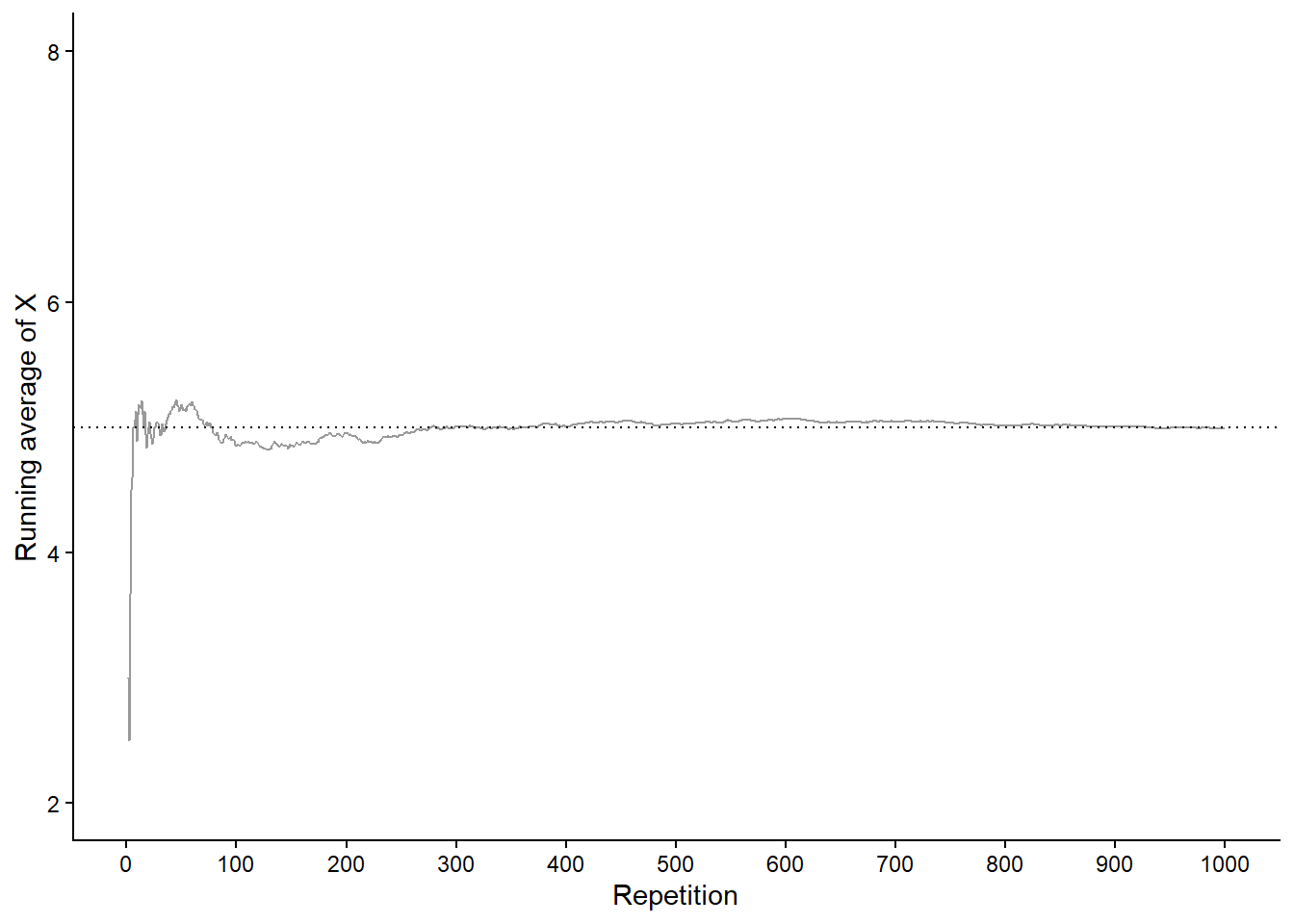
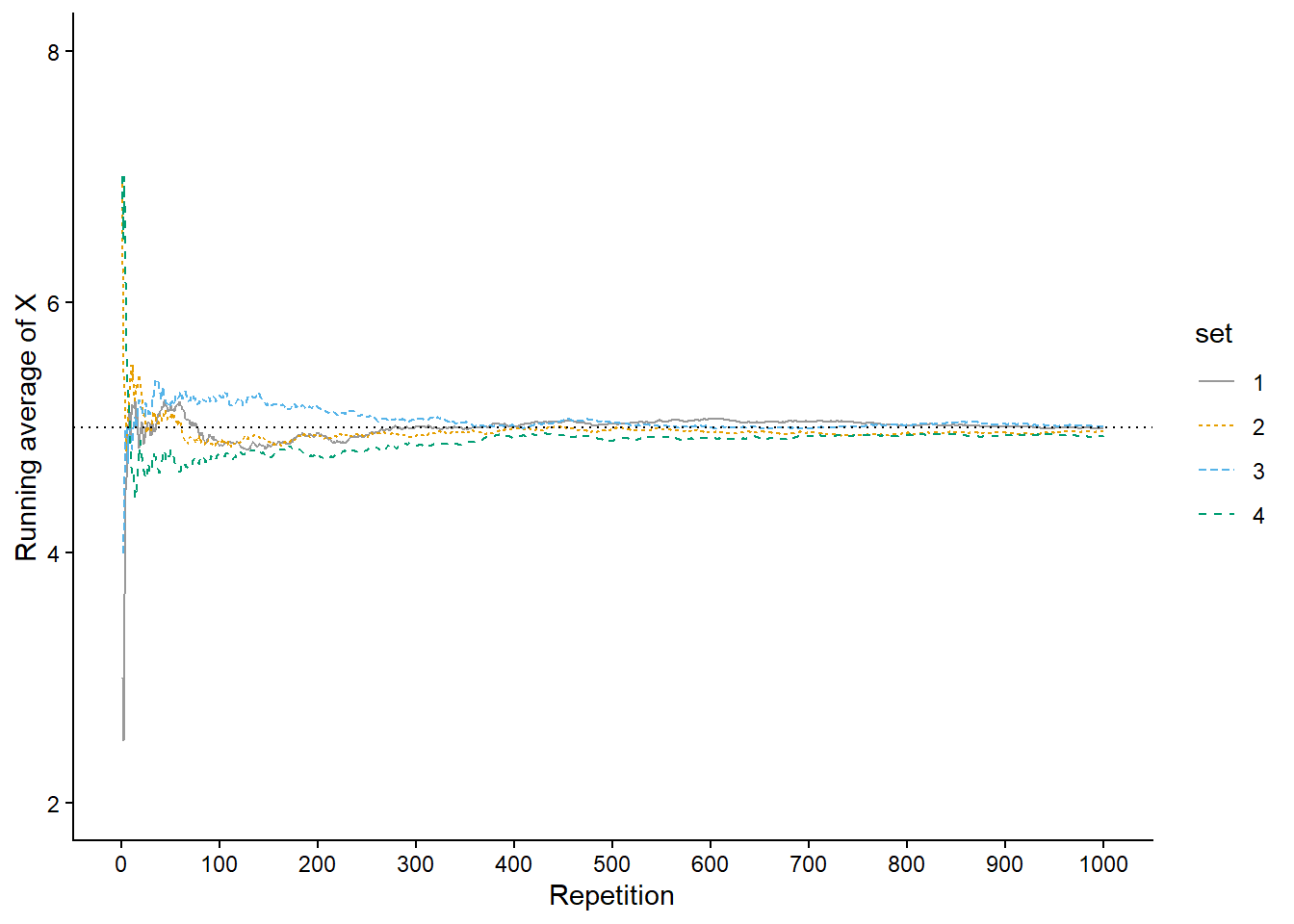
(a) A single simulation of 1000 pairs of rolls

The marginal distribution of $X$, depicted in Figure 2.16, shows that 5 is the “balance point” of the distribution. In Example 2.44 we saw that 5 is the probability-weighted average value of $X$, and we interpreted 5 as the value of $X$ we would “expect” to see on average in the long run. In this sense, 5 is the “true” long run average value of $X$, and our simulation results agree. We will discuss later “true” long run average values or “expected values” in much more detail later. For now, we’ll rely on simulation: we can approximate the long run average value of a random variable $X$ by simulating many values of $X$ and finding the average in the usual way.

Recall that a probability is a theoretical long run relative frequency. A probability can be approximated by a relative frequency from a large number of simulated repetitions, but there is some simulation margin of error.

Likewise, the average value of $X$ after a large number of simulated repetitions is only an approximation to the theoretical long run average value of $X$, and there is margin of error due to natural variability in the simulation. The margin of error is also on the order of $1/\sqrt{N}$ where $N$ is the number of independently simulated values used to compute the average. However, the degree of variability of the random variable itself also influences the margin of error when approximating long run averages. In particular, if $\sigma$ is the standard deviation (see Section 3.8) of the random variable, then the margin of error for the average is on the order of $\sigma / \sqrt{N}$.

Remember that the long run average value is just one feature of a marginal distribution. There is much more to the long run pattern of variability of a random variable than just its average value. We are also interested in percentiles, degree of variability, and quantities that measure relationships between random variables. Two random variables can have the same long run average value but very different distributions. For example, the average temperature in both Phoenix, AZ and Miami, FL is around 75 degrees F, but the distribution of temperatures is not the same.

3.7.3 Averages in Symbulate

Continuing Example 3.10 let $X$ be the sum of two rolls of a fair four-sided die. In Symbulate, we first simulate and store 10000 values of $X$.

P = BoxModel([1, 2, 3, 4], size = 2)

X = RV(P, sum)

x = X.sim(10000)

We can approximate the long run average value of $X$ by computing the average—a.k.a., mean—of the 10000 simulated values in the usual way: sum the 10000 simulated values stored in x and divide by 10000. Here are a few ways of computing the mean of the simulated values.

x.sum() / 10000

4.9833

x.sum() / x.count()

4.9833

x.mean()

4.9833

Averages are computed the same way, regardless of whether the variable is discrete or continuous. The following code computes the average of 5 then 10000 simulated values of $X$, a random variable with the Normal(30, 10) distribution from Section 3.2.2.

X = RV(Normal(30, 10))

x = X.sim(5)

x

Index	Result
0	39.71625520756501
1	33.01924481847947
2	44.69724172857143
3	33.99830783036135
4	34.5067985870937

x.mean()

37.187569634414196

x = X.sim(10000)

x

Index	Result
0	13.043632846080147
1	25.71164225043016
2	14.29280816239234
3	44.26852374230779
4	36.27232542792389
5	22.934414450007438
6	9.59902733091283
7	30.636970350344924
8	14.073178395254358
...	...
9999	21.648706983654534

x.mean()

30.076043607021983

Our simulation suggests that the long run average of a random variable with a Normal(30, 10) distribution is approximately 30. In general, one parameter of a Normal distribution represents its expected value, a.k.a., (long run) mean; the other parameter represents its standard deviation, which we will discuss soon (in Section 3.8).

3.7.4 Linearity of averages

Now we’ll introduce a useful properties of averages.

Example 3.13 Recall your tactile simulation from Example 3.5). Let $U_1$ be the result of the first roll, and $U_2$ the result of the second, so the sum is $X = U_1 + U_2$.

Donny Don’t says: “$X=U_1+U_2$, so I can find the average value of $X$ by finding the average value of $U_1$, the average value of $U_2$, and adding the two averages”. Do you agree? Explain.
Donny Don’t says: “$U_1$ and $U_2$ have the same distribution, so they have the same average value, so I can find the average value of $X$ by multiplying the average value of $U_1$ by 2”. Do you agree? Explain.
Donny Don’t says: “$U_1$ and $U_2$ have the same distribution, so $X=U_1+U_2$ has the same distribution as $2U_1 = U_1 + U_1$”. Do you agree? Explain.

Solution (click to expand)

Solution 3.13.

Donny is correct! Our simulation results are in Table 3.10. The average value of $U_1$ is \[ \frac{2 + 1 + 3 + 4 + 3 + 3 + 2 + 2 + 1 + 3}{10} = 2.4 \] The average value of $U_2$ is \[ \frac{1 + 1 + 3 + 3 + 2 + 4 + 3 + 4 + 2 + 4}{10} = 2.7 \] The sum of these two values is equal to the average value of $X$. To see why, suppose we had just performed two repetitions, resulting in the last two rows of Table 3.10). \[ {\scriptsize \text{Average of $(U_1+U_2)$} = \frac{(1 + 2) + (3 + 4)}{2} = 5 = 2 + 3= \left(\frac{1 + 3}{2}\right)+\left(\frac{2 + 4}{2}\right) = (\text{Average of $U_1$}) + (\text{Average of $U_1$}) } \] We discuss further below.
Donny is correct that $U_1$ and $U_2$ have the same distribution, and he has some good ideas about averages. But we should remind Donny that a distribution represents the long run pattern of variability. With only 10 repetitions, the results for $U_1$ will not necessarily follow the same pattern as those for $U_2$. In our simulation, the average value of $U_1$ is 2.4 and the average value of $U_2$ is 2.7. Multiplying neither one of these numbers by 2 yields the average value of $X$. Donny would have been correct if he were talking about long run average values. Since $U_1$ and $U_2$ have the same distribution, the long run average value of $U_1$ is equal to the long run average value of $U_2$, and so the long run average value of $X$ is equal to the long run average value of $U_1$ multiplied by two.
Donny is not correct. In particular, $X$ and $2U_1$ do not have the same possible values; for example, $X$ can be 3 but $2U_1$ cannot. The long run average value is just one feature of a distribution. Just because $X$ and $2U_1$ have the same long run average value does not necessarily mean they have the same full long run pattern of variability. In particular, relationships between random variables will affect distributions of transformations of them. $U_1$ and $U_2$ have the same marginal distribution, but the joint distribution of $(U_1, U_2)$ is not the same as that of $(U_1, U_1)$, and so the distribution of $U_1+U_2$ is not the same as that of $U_1+U_1$.

In general the order of transforming and averaging is not interchangeable. However, the order is interchangeable for linear transformations.

Theorem 3.1 (Linearity of averages) If $X$ and $Y$ are random variables and $m$ and $b$ are non-random constants, whether in the short run or the long run,

\[\begin{align*} \text{Average of $(mX+b)$} & = m(\text{Average of $X$})+b\\ \text{Average of $(X+Y)$} & = \text{Average of $X$} +\text{Average of $Y$} \end{align*}\]

The following just restates in terms of long run averages (expected values)

Theorem 3.2 (Linearity of expected value) If $X$ and $Y$ are random variables and $m$ and $b$ are non-random constants,

\[\begin{align*} \textrm{E}(mX+b) & = m\textrm{E}(X)+b\\ \textrm{E}(X+Y) & = \textrm{E}(X) + \textrm{E}(Y) \end{align*}\]

For example, if $X$ measures temperature in degrees Celsius with average 24°C, then $1.8X+32$ measures temperature in degrees Fahrenheit with average 75.2°F.

Averaging involves adding and dividing. Linear transformations involve only adding/subtracting and multiplying/dividing. The ability to interchange the order of averaging and linear transformations follows simply from basic properties of arithmetic (commutative, associative, distributive).

Note that the average of the sum of $X$ and $Y$ is the sum of the average of $X$ and the average of $Y$ regardless of the relationship between $X$ and $Y$. We will explore this idea in more detail later.

3.7.5 Averages of indicator random variables

Recall that indicators are the bridge between events and random variables. Indicators are also the bridge between relative frequencies and averages.

Example 3.14 Recall your tactile simulation from Example 3.5. Let $A$ be the event that the first roll is 3 and $\textrm{I}_A$ the corresponding indicator random variable. Based only on the results of your simulation, approximate the long run average value of each of $\textrm{I}_A$. What do you notice?

Solution (click to expand)

Solution 3.14. Our simulation results are in Table 3.10. Approximate the long run average value of $\textrm{I}_A$ by summing the 10 simulated values of $\textrm{I}_A$ and dividing by 10. \[ \frac{0 + 0 + 1 + 0 + 1 + 1 + 0 + 0 + 0 + 1}{10} = \frac{4}{10} \] The average of $\textrm{I}_A$ is the relative frequency of event $A$! When we sum the 1/0 values of $\textrm{I}_A$ we count the repetitions on which $A$ occurs. That is, the numerator in the average calculation for $\textrm{I}_A$ is the frequency of event $A$, and dividing by the number of repetitions yields the relative frequency of event $A$.

If $\textrm{I}_A$ is the indicator random variable of an event $A$, whether in the short run or the long run, \[ \text{Average of $\textrm{I}_A$} = \text{Relative frequency of $A$} \] In terms of our long run notation, the above long run result is \[ \textrm{E}(\textrm{I}_A) = \textrm{P}(A) \]

Indicators provide a bridge between events and random variables, and between probability and expected value.

3.7.6 Exercises

Exercise 3.18 Suppose that a total of 350 students at a college are taking a particular statistics course. The college offers five sections of the course, each taught by a different instructor. The class sizes are shown in the following table.

Section	A	B	C	D	E
Number of students	35	35	35	35	210

We are interested in: What is the average class size?

Suppose we randomly select one of the 5 instructors. Let $X$ be the class size for the selected instructor. Specify the distribution of $X$. (A table is fine.)
Compute and interpret $\text{E}(X)$.
Compute and interpret $\text{P}(X = \text{E}(X))$.
Suppose we randomly select one of the 350 students. Let $Y$ be the class size for the selected student. Specify the distribution of $Y$. (A table is fine.)
Compute and interpret $\text{E}(Y)$.
Compute and interpret $\text{P}(Y = \text{E}(Y))$.
Comment on how these two expected values compare, and explain why they differ as they do. Which average would you say is more relevant?

Exercise 3.19 The latest series of collectible Lego Minifigures contains 3 different Minifigure prizes (labeled 1, 2, 3). Each package contains a single unknown prize. Suppose we only buy 3 packages and we consider as our sample space outcome the results of just these 3 packages (prize in package 1, prize in package 2, prize in package 3). For example, 323 (or (3, 2, 3)) represents prize 3 in the first package, prize 2 in the second package, prize 3 in the third package. Let $X$ be the number of distinct prizes obtained in these 3 packages. Let $Y$ be the number of these 3 packages that contain prize 1.

Explain how you could, in principle, conduct a simulation by hand and use the results to approximate
1. $\textrm{E}(X)$
2. $\textrm{E}(Y)$
3. $\textrm{E}(X^2)$
4. $\textrm{E}(XY)$
Write Symbulate code to conduct a simulation and approximate the values in part 1.

Exercise 3.20 Consider a continuous version of the dice rolling problem where instead of rolling two fair four-sided dice (which return values 1, 2, 3, 4) we spin twice a Uniform(1, 4) spinner (which returns any value in the continuous range between 1 and 4). Let $X$ be the sum of the two spins and let $Y$ be the larger of the two spins.

Describe in words how you could use simulation to approximate
1. $\textrm{E}(X)$
2. $\textrm{E}(Y)$
3. $\textrm{E}(X^2)$
4. $\textrm{E}(XY)$
Write Symbulate code to conduct a simulation to approximate the quantities in part 1.

3.8 Measuring variability: Variance and standard deviation

The long run average value is just one feature of a distribution. Random variables vary, and the distribution describes the entire pattern of variability. It is also convenient to measure the overall degree of variability in a single number. Some values of a variable are close to its mean and some are far, so to measure variability in a single number we might ask: how far are the values away from the mean on average? Variance and standard deviation are numbers that address this question.

Consider again a random variable $X$ that follows a Normal(30, 10) distribution; we’ll assume $X$ is measured in minutes (after noon) as in the meeting problem. Any Normal distribution has two parameters, the mean and the standard deviation; the Normal(30, 10) distribution has mean 30 (minutes) and standard deviation 10 (minutes). In Section 3.7.3 we saw simulation evidence supporting that the mean is 30. Now we’ll investigate the standard deviation, which measures, roughly, the average distance from the mean.

We’ll motivate the calculation of standard deviation using using just the 10 simulated values in Table 3.5, reproduced in Table 3.12. For now focus on only the first three columns of Table 3.12. We see how far a value is away from the mean by subtracting the mean, resulting in a “deviation”. Deviations are positive for values that are above the mean and negative for values that are below the mean. For example, the value 21.387 is 11.973 minutes below the mean.

Table 3.12: Calculation of standard deviation based on 10 simulated values

repetition	x	deviation	absolute_deviation	squared_deviation
1	21.387	-11.973	11.973	143.345
2	50.719	17.359	17.359	301.347
3	24.090	-9.270	9.270	85.940
4	32.680	-0.680	0.680	0.462
5	54.511	21.151	21.151	447.347
6	38.117	4.757	4.757	22.629
7	16.819	-16.541	16.541	273.619
8	22.980	-10.380	10.380	107.746
9	28.867	-4.493	4.493	20.187
10	43.430	10.070	10.070	101.411
Sum	333.600	0.000	106.674	1504.033
Average	33.360	0.000	10.667	150.403

We might try to compute the average deviation from the mean, but this will always be 0. The mean is the balance point—that is, the center of gravity—so the (positive) deviations above the mean will always balance out, in total, with the (negative) deviations below the mean. However, regarding degree of variability, we only care about how far values are away from the mean, not if they’re above or below. So we take the absolute value of each deviation and then find the average. See the fourth column of Table 3.12, resulting in an average absolute deviation of 10.667 minutes.

Table 3.12 motivates the calculation, but we’re really interested in what happens in the long run, so let’s carry out the calculation for many simulated values.

X = RV(Normal(30, 10))

x = X.sim(10000)

x

Index	Result
0	30.854701264223483
1	32.18602451516775
2	26.01404843627838
3	21.8079119347735
4	38.252372928854456
5	32.67591315368069
6	58.49606025356133
7	40.907900857524616
8	32.90324622476121
...	...
9999	24.140614903236216

The mean is about 30.

x.mean()

29.951495449842653

Now we compute the absolute deviations from the mean.

abs(x - x.mean())

Index	Result
0	0.9032058143808293
1	2.2345290653250984
2	3.937447013564274
3	8.143583515069153
4	8.300877479011803
5	2.7244177038380357
6	28.54456480371868
7	10.956405407681963
8	2.9517507749185583
...	...
9999	5.8108805466064375

Then we average the absolute deviations.

abs(x - x.mean()).mean()

8.023974860792508

Unfortunately, the above calculation yields roughly 8 rather than the standard deviation of 10. It turns out that for a Normal(30, 10) distribution the long run average absolute deviation from the mean is about 8. We can conceptualize standard deviation as average distance from the mean, but the actual calculation of standard deviation is a little more complicated. Technically, we must first square all the distances and then average; the result is the variance. Then the square root of the variance is the standard deviation³¹.

\[\begin{align*} \text{Variance of } X & = \text{Average of } [(X - \text{Average of } X)^2]\\ \text{Standard deviation of } X & = \sqrt{\text{Variance of } X} \end{align*}\]

Returning to the 10 simulated values in Table 3.12, the fifth column contains the squared deviations. Notice that squaring the deviations has a similar effect to taking the absolute value: a value that is 3 units above the mean has the same squared deviation as a value that is 3 units below the mean (since $3^2 = (-3)^2$). Now we average the squared deviations to obtain the variance. The average is computed in the usual way: sum all the values and divide by the number of values³². But now each value included in the average is the squared deviation of $X$ from the mean, rather than the value of $X$ itself. The variance of the 10 simulated values is 150.403. This probably seems like a weird number, and it is: because we squared all the deviations before averaging, the measurement units of the variance are minutes². To get back to the original measurement units, we take the square root of the variance, $\sqrt{150.403}$, resulting in the standard deviation of 12.264 minutes.

Now back to the long run, using 10000 simulated values x. The following code shows the “long way” of computing variance and standard deviation. First, find the squared distance between each simulated value and the mean.

(x - x.mean()) ** 2

Index	Result
0	0.815780743131337
1	4.993120143782658
2	15.50348898462622
3	66.31795246690606
4	68.90456692156533
5	7.422451824986115
6	814.7921798336952
7	120.04281945748257
8	8.71283263723231
...	...
9999	33.76633272692913

Then compute the average squared deviation to get the variance.

((x - x.mean()) ** 2).mean()

100.53603867646262

Now take the square root of the variance to get the standard deviation.

sqrt(((x - x.mean()) ** 2).mean())

10.026766112583989

We see that the standard deviation is about 10—as it should be for values simulated from a Normal(30, 10) distribution—and the variance is about $10^2 = 100$. Fortunately, var and sd will carry out these calculations more quickly.

x.var()

100.53603867646262

x.sd()

10.026766112583989

Example 3.15 We’ll compare long run average and standard deviation for the Uniform(0, 60) distribution and the Normal(30, 10) distribution.

Make an educated guess for the long run average value of a Uniform(0, 60) distribution.
Will the standard deviation for a Uniform(0, 60) distribution be greater than, less than, or equal to 10, the standard deviation for a Normal(30, 10) distribution? Explain without doing any calculations. (Hint: It might help to compare the spinners in Section 3.2 or the simulations from Section 3.4.)
Make an educated guess for the standard deviation of a Uniform(0, 60) distribution.

Solution (click to expand)

Solution 3.15.

It seems reasonable that the long run average value of a Uniform(0, 60) distribution is 30, the balance point of the distribution.
While the Uniform(0, 60) and Normal(30, 10) distributions have the same mean of 30, the Uniform(0, 60) has a larger standard deviation than the Normal(30, 10) distribution. In comparison to a Normal(30, 10) distribution, a Uniform(0, 60) distribution will give higher probability to ranges of values near the extremes of 0 and 60, as well as lower probability to ranges of values near 30. Thus, there will be more values far from the mean of 30 and fewer values close, and so the average distance from the mean and hence standard deviation will be larger for the Uniform(0, 60) distribution than for the Normal(30, 10) distribution. See Figure 3.22 which compares histograms of simulated values from the two distributions.
In a Uniform(0, 60) distribution, values are “evenly spread” from 0 to 60, so distances from the mean are “evenly spread” from 0 (for 30) to 30 (for 0 and 60). We might expect the standard deviation—roughly the average distance from the mean—to be about 15, halfway between 0 and 30. It turns out that the standard deviation is about 17; 15 is the average absolute deviation from the mean. While the “average distance” interpretation helps our conceptual understanding of standard deviation, the process of squaring the distances, then averaging, and then taking the square root makes guessing the actual value of standard deviation difficult.

U = RV(Uniform(0, 60))

u = U.sim(10000)

plt.figure()

x.plot()
u.plot()

plt.legend(['Normal(30, 10)', 'Uniform(0, 60)']);
plt.show()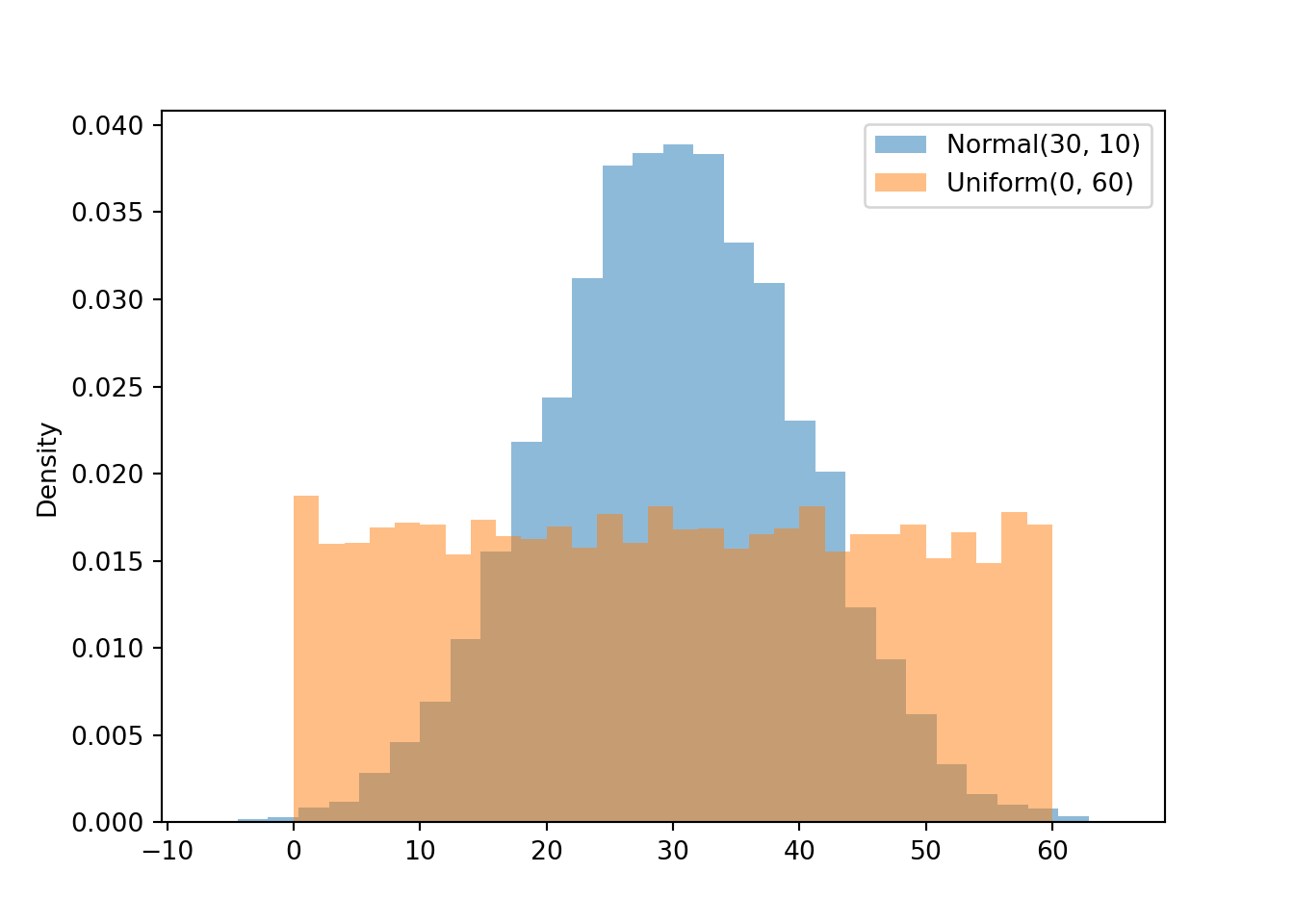

Figure 3.22: Histograms of many simulated values from each of the Normal(30, 10) and Uniform(0, 60) distributions.

u.sd()

17.339948595579052

abs(u - u.mean()).mean()

14.98714087463523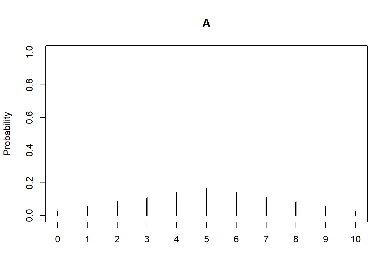

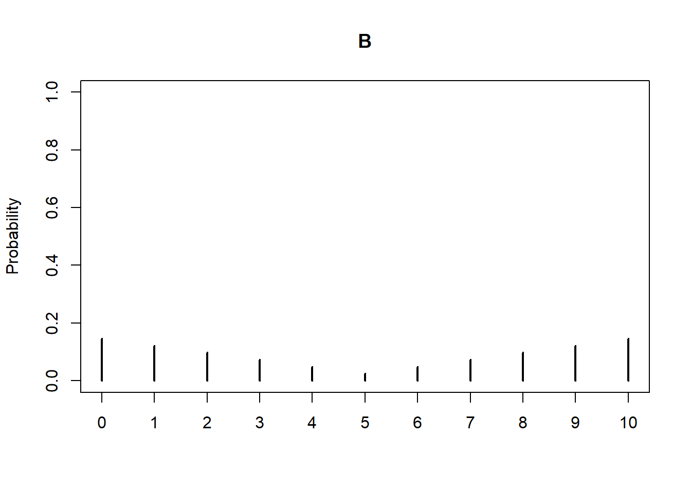
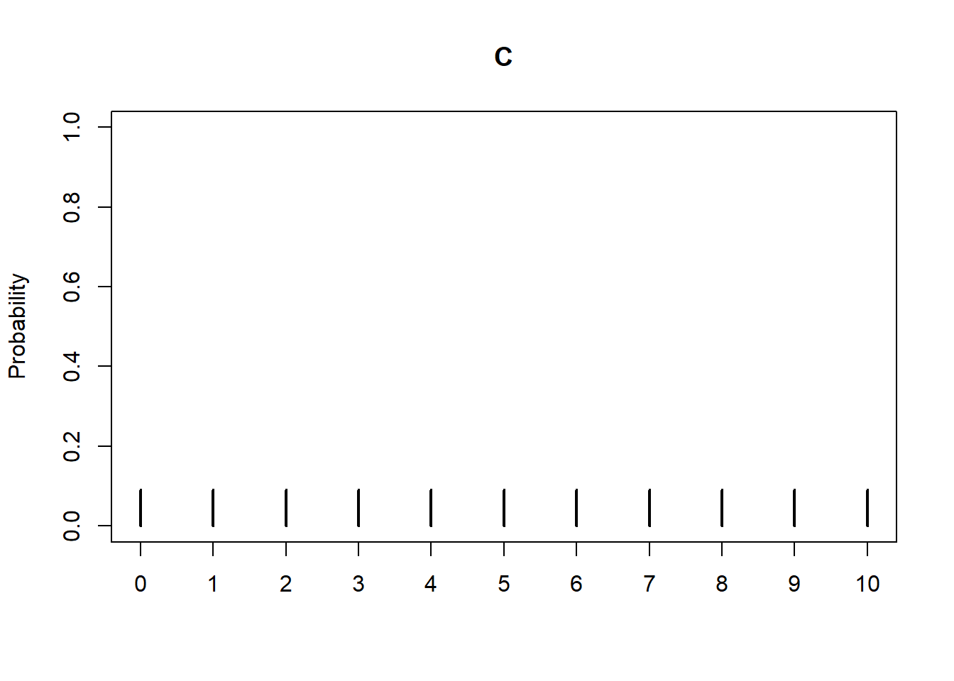
Example 3.16 The plots below summarize hypothetical distributions of quiz scores in six classes. Each quiz score is a whole number between 0 and 10 inclusive. All plots are on the same scale with quiz scores on the horizontal axis, and probability on the vertical axis.

Donny Dont says that of these six plots, C represents the smallest SD, since there is “no variability in the heights of the bars”. Do you agree that C represents “no variability”? Explain.
What is the smallest possible value the SD of quiz scores could be? What would need to be true about the distribution for this to happen? (This scenario might not be represented by one of these six plots.)
Without doing any calculations, identify which of these six classes exhibits the smallest standard deviation of quiz scores.
Without doing any calculations, arrange the classes in order based on their standard deviations from smallest to largest.
In one of the classes, the standard deviation of quiz scores is 5. Which one? Why?
Is the standard deviation in F greater than, less than, or equal to 1? Why?
Provide a ballpark estimate of standard deviation in each case.

Solution (click to expand)

Solution 3.16.

We disagree with Donny. Standard deviation measures variability of the values of the variable, not their probabilities. If we were to simulate values according to the distribution in C, we would observe some 0s, some 1s, some 2s, all the way through some 10s (with roughly equal frequency). So there would certainly be variability in the values of the variable. Remember that values of the variable are along the horizontal axis, so standard deviation measures average distance from the mean horizontally.
The smallest possible value of standard deviation is 0, which occurs only if the random variable is a constant (with probability 1). In this context, if every student had the same quiz score, e.g., if 100% of students scored an 8, then the standard deviation would be 0. The distribution plot would have a single spike at a single value.
Remember that values of the variable are along the horizontal axis, so standard deviation measures average distance from the mean horizontally. The distribution in F represents the smallest standard deviation. The mean is 7, most of the scores are 7, and some of the scores are only 1 unit away from the mean. In all other situations, the probability that the random variable is equal to its mean is smaller, and the probability that the random variables takes a value more than 1 unit away from its mean is larger than in F.
In all plots other than F the mean is 5, so the smallest standard deviation occurs where the values tend to be close to 5, and the largest occurs where the values tend to be far from 5. In order from smallest to largest standard deviation: F, E, A, C, B, D.
In D, the score takes values 0 and 10 with probability 0.5. The mean is 5, and all deviations are 5 units away from the mean, so the average squared deviation will be $5^2$ and the standard deviation will be 5.
Less than 1. Don’t forget that there is a high probability of a deviation of 0 in this case. So the average deviation will be somewhere between 0 and 1.
Some of these are harder than others. In E, many values are 0 units away from mean, many values are 1 unit away, and some values are 2. So the standard deviation in E is maybe around 1. In C, there are values that are 0 units away, and about as many values that are each 1, 2, 3, 4, and 5 units away; we might expect standard deviation to be around 2.5. But remember, while considering the average absolute deviation helps intuition, standard deviation is actually the square root of the average squared deviation so the exact value can be difficult to ascertain without computation. The actual values are: F = 0.45, E = 1.15, A = 2.4, C = 3.1, B = 3.7, D = 5.

Variance and standard deviation are both based on average squared deviations from the mean. Variance has some nice mathematical properties (which we’ll see later), but standard deviation is the more “practical” number since it has the same measurement units as the variable. In computations we often work with variances then take the square root at the end to report and interpret standard deviations.

Standard deviation is the most commonly used single-number measure of variability, but it’s not the only one. Average absolute deviation also measures variability; why not use that? It turns out that squaring deviations, rather than taking absolute values, leads to nicer mathematical properties³³. Also, standard deviation is the natural measure of variability for Normal distributions (we’ll investigate why later). While standard deviation is commonly used, there are other, sometimes better, ways to summarize variability. For example, we will see later how percentiles can be used to summarize the pattern of variability.

The following definiton states our notion of variance in expected value terms.

Definition 3.1 (Variance and standard deviation of a random varible) The variance of a random variable $X$ is \[ \textrm{Var}(X) = \textrm{E}((X-\textrm{E}(X))^2) \] The standard deviation of a random variable $X$ is $\textrm{SD}(X) = \sqrt{\textrm{Var}(X)}$.

Recall that an expected value is a long run average. Thefore we can interpret $\textrm{E}(\cdot)$ as “simulate many values of what’s inside $(\cdot)$ and average”. In this way \[ \textrm{E}((X-\textrm{E}(X))^2) = \text{Long Run Average of } [(X - \text{Long Run Average of } X)^2] \]

Recall that for discrete random variables we can compute expected values as probability-weighted average values. We can compute variances for discrete random variables in a similar way.

Example 3.17 In the dice rolling problem, let $Y$ be the larger of the two rolls. The marginal distribution of $Y$ is represented by Table 2.15. In Example 2.44 we computed $\textrm{E}(Y) = 3.125$.

Compute $\textrm{Var}(Y)$.
Compute $\textrm{SD}(Y)$.
Describe in detail how $\textrm{Var}(Y)$ can be simulated via approximation
Write Symbulate code to approximate $\textrm{Var}(Y)$ and $\textrm{SD}(Y)$ and compare to the values from parts 1 and 2.

Solution (click to expand)

Solution 3.17.

$Y$ takes values 1, 2, 3, 4, and $\textrm{E}(Y)=3.125$, so $(Y-\textrm{E}(Y))^2$ takes values $(1-3.125)^2$, $(2-3.125)^2$, $(3-3.125)^2$, $(4-3.125)^2$, with respective probability 1/16, 3/16, 5/16, 7/16. To compute $\textrm{E}((Y-\textrm{E}(Y))^2)$ as a probability-weighted average value, multiply each possible of $(Y-\textrm{E}(Y))^2$ by its probability and sum. \[ (1-3.125)^2\times 0.0625 + (2-3.125)^2 \times 0.1875 + (3-3.125)^2 \times 0.3125 + (4-3.125)^2 \times 0.4375 = 0.8594 \] See Table 3.13 for more detail. $\textrm{Var}(Y) = 0.8594$.
$\textrm{SD}(Y)=\sqrt{\textrm{Var}(Y)} = \sqrt{0.8594} = 0.9270$.
We have already discussed how to simulate a value of $Y$ in this content. To approximate the variance
- Simulate many values of $Y$
- Compute the average of the simulated values of $Y$ (to approximate $\textrm{E}(Y)$)
- From each simulated value of $Y$ subtract the average, and then square
- Compute the average of the squared deviations from the previous part to approximate the variance
See below for the code, both the long way and using the var and sd shortcuts. The simulation-based approximations are close to the values from parts 1 and 2.

Table 3.13: Steps in computing the variance of $Y$ in Example 3.17.

$y$	$y - \textrm{E}(Y)$	$(y - \textrm{E}(Y))^2$	$\textrm{P}(Y=y)$	$(y - \textrm{E}(Y))^2\textrm{P}(Y=y)$
1	-2.125	4.5156	0.0625	0.2822
2	-1.125	1.2656	0.1875	0.2373
3	-0.125	0.0156	0.3125	0.0049
4	0.875	0.7656	0.4375	0.3350

P = BoxModel([1, 2, 3, 4], size = 2)

Y = RV(P, max)

y = Y.sim(10000)

y

Index	Result
0	4
1	4
2	2
3	3
4	4
5	4
6	2
7	4
8	2
...	...
9999	4

y.mean()

3.1071

y - y.mean()

Index	Result
0	0.8929
1	0.8929
2	-1.1071
3	-0.10709999999999997
4	0.8929
5	0.8929
6	-1.1071
7	0.8929
8	-1.1071
...	...
9999	0.8929

(y - y.mean()) ** 2

Index	Result
0	0.7972704100000001
1	0.7972704100000001
2	1.22567041
3	0.011470409999999993
4	0.7972704100000001
5	0.7972704100000001
6	1.22567041
7	0.7972704100000001
8	1.22567041
...	...
9999	0.7972704100000001

((y - y.mean()) ** 2).mean()

0.87162959

y.var()

0.87162959

y.sd()

0.9336110485635868

Example 3.18 Continuing Example 3.17.

Compute $\textrm{E}(Y^2)$.
Describe in detail how $\textrm{E}(Y^2)$ can be approximated via simulation.
Compute $\textrm{E}(Y^2) - (\textrm{E}(Y))^2$. What do you notice?

Solution (click to expand)

Solution 3.18.

$Y$ takes values 1, 2, 3, 4, so $Y^2$ takes values $1^2, 2^2, 3^2, 4^2$, with respective probability 1/16, 3/16, 5/16, 7/16. To compute $\textrm{E}(Y^2)$ as a probability-weighted average value, multiply each possible of $Y^2$ by its probability and sum. \[ 1^2\times 0.0625 + 2^2 \times 0.1875 + 3^2 \times 0.3125 + 4^2 \times 0.4375 = 10.625 \] $\textrm{E}(Y^2) = 10.625$. Notice this is not the same as $\textrm{E}(Y)^2=3.125^2.$
We have already discussed how to simulate a value of $Y$ in this content. To approximate $\textrm{E}(Y^2)$
- Simulate many values of $Y$
- Square each simulated value of $Y$
- Compute the average of the squared values from from the previous part to approximate $\textrm{E}(Y^2)$. See the Symbulate code below.
$\textrm{E}(Y^2) - (\textrm{E}(Y))^2 = 10.625 - 3.125^2 = 0.8594$, which is $\textrm{Var}(Y)$.

(y ** 2)

Index	Result
0	16
1	16
2	4
3	9
4	16
5	16
6	4
7	16
8	4
...	...
9999	16

(y ** 2).mean()

10.5257

(y ** 2).mean() - (y.mean()) ** 2

0.8716295900000013

Example 3.18 illustrates an alternative formula for computing variance. Definition 3.1 represents the concept of variance. However, variance is usually computed using the following equivalent but slightly simpler formula.

Lemma 3.1 \[ \textrm{Var}(X) = \textrm{E}(X^2) - (\textrm{E}(X))^2 \]

That is, the variance of $X$ is the expected value of the square of $X$ minus the square of the expected value of $X$.

We will see that variance has many nice theoretical properties. Whenever you need to compute a standard deviation, first find the variance and then take the square root at the end.

We will see how to compute variance for continuous random variables later. But Definition 3.1 and Lemma 3.1 apply for both discrete and continuous random variables. Furthermore, variance can be approximated via simulation in the same way for discrete or continuous random variables: simulate many values of the random variable and compute the average of the squared deviations from the mean.

3.8.1 Standardization

Standard deviation provides a “ruler” by which we can judge a particular value of a random variable relative to the distribution of values. This idea is particularly useful when comparing random variables with different measurement units but whose distributions have similar shapes.

Example 3.19 SAT scores have, approximately, a Normal distribution with a mean of 1050 and a standard deviation of 200. ACT scores have, approximately, a Normal distribution with a mean of 21 and a standard deviation of 5.5. Darius’s score on the SAT is 1500. Alfred’s score on the ACT is 31. We’ll investigate who scored relatively better on their test.

Compute the deviation from the mean for Darius’s SAT score. How large is this value relative to the standard deviation for SAT scores (which measures, roughly, the average deviation from the mean)?
Compute the deviation from the mean for Alfred’s ACT score. How large is this value relative to the standard deviation for ACT scores?
Who scored relatively better on their test? Explain.

Solution (click to expand)

Solution 3.19.

Darius’s score is $1500-1050 = 450$ points above the mean SAT score. The standard deviation of SAT scores is 200 points. Roughly, the deviation of Darius’s score from the mean is $450/200 = 2.25$ times larger the average deviation.
That is, Darius’s SAT score of 1500 is 2.25 standard deviations above the mean SAT score.
Alfred’s score is $31-21 = 10$ points above the mean ACT score. The standard deviation of ACT scores is 5.5 points. Roughly, the deviation of Alfred’s score from the mean is $10/5.5 = 1.82$ times larger than the average deviation. That is, Alfred’s ACT score of 31 is 1.82 standard deviations above the mean ACT score.
Both scores are above average, but relative to other test scores, Darius’s is farther above average than Alfred’s. Both distributions are Normal, so the probability that an SAT score is greater than Darius’s is smaller than the probability that an ACT score is greater than Alfred’s. That is, Darius scored relatively better. See Figure 3.29.

Figure 3.29: Comparison of the Normal distributions in Example 3.19.

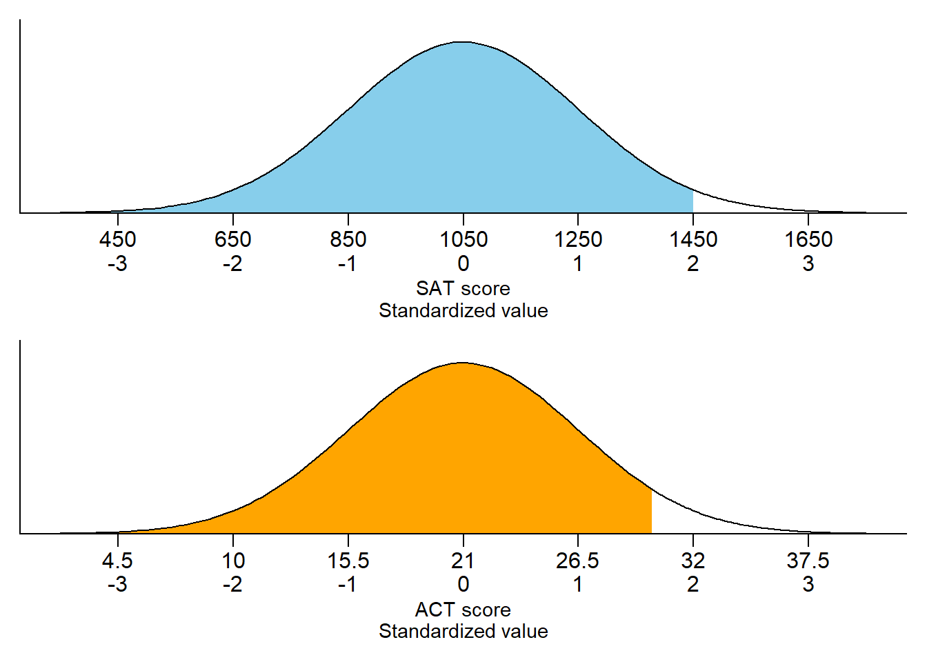
Standard deviation provides a “ruler” by which we can judge a particular value of a random variable relative to the distribution of values. Consider the plot for SAT scores in Figure 3.29. For now, pay attention to the two horizontal axis scales on each plot; we’ll discuss the Normal “bell shape” in more detail later. There are two scales on the variable axis: one representing the actual measurement units, and one representing “standardized units”. In the standardized scale, values are measured in terms of standard deviations away from the mean:

The mean corresponds to a value of 0.
A one unit increment on the standardized scale corresponds to an increment equal to the standard deviation in the measurement unit scale.

For example, each one unit increment in the standardized scale corresponds to a 200 point increment in the measurement unit scale for SAT scores, and a 5.5 point increment in the measurement unit scale for ACT scores. An SAT score of 1250 is “1 standard deviation above the mean”; an ACT score of 10 is “2 standard deviations below the mean”. Given a specific distribution, the more standard deviations a particular value is away from its mean, the more extreme or “unusual” it is.

Given a value of a variable, its standardized value marks where the value lies on the standardized scale (e.g., 1500 on the SAT scale corresponds to 2.25 on the standardized scale).

\[ \text{Standardized value} = \frac{\text{Value - Mean}}{\text{Standard deviation}} \]

Warning

Standardization is useful when comparing random variables with different measurement units but whose distributions have similar shapes (like the two Normal distributions in Figure 3.29). However, standardized values are only based on two features of a distribution—mean and standard deviation—rather than the complete pattern of variability. Distributions with different shapes have different patterns of variability. We will see later than when comparing distributions with different shapes, it is better to compare percentiles rather than standardized values to determine what is “extreme” or “unusual”.

Any random variable can be standardized, but keep in mind that just how extreme any particular standardized value is depends on the shape of the distribution. We will see that standardization is most natural for random variables that follow a Normal distribution.

3.8.2 Normal distributions (briefly)

Standardization is most natural for random variables that follow a Normal distribution. The Normal(30, 10) model that we assumed for arrival times in the meeting problem is an example of a Normal distribution. The pattern of variability for any Normal distribution follows a particular bell shape, like in Figure 3.29. A Normal distribution has two parameters: its mean (typically denoted $\mu$) and its standard deviation (typically denoted $\sigma$). For Normal distributions the probability that a value is within (or beyond) a given number of standard deviations from the mean follows a specific pattern called the “empirical rule”. For example, the empirical rule for Normal distributions specifies that

68% of values are within 1 standard deviation of the mean
95% of values are within 2 standard deviations of the mean
99.7% of values are within 3 standard deviations of the mean

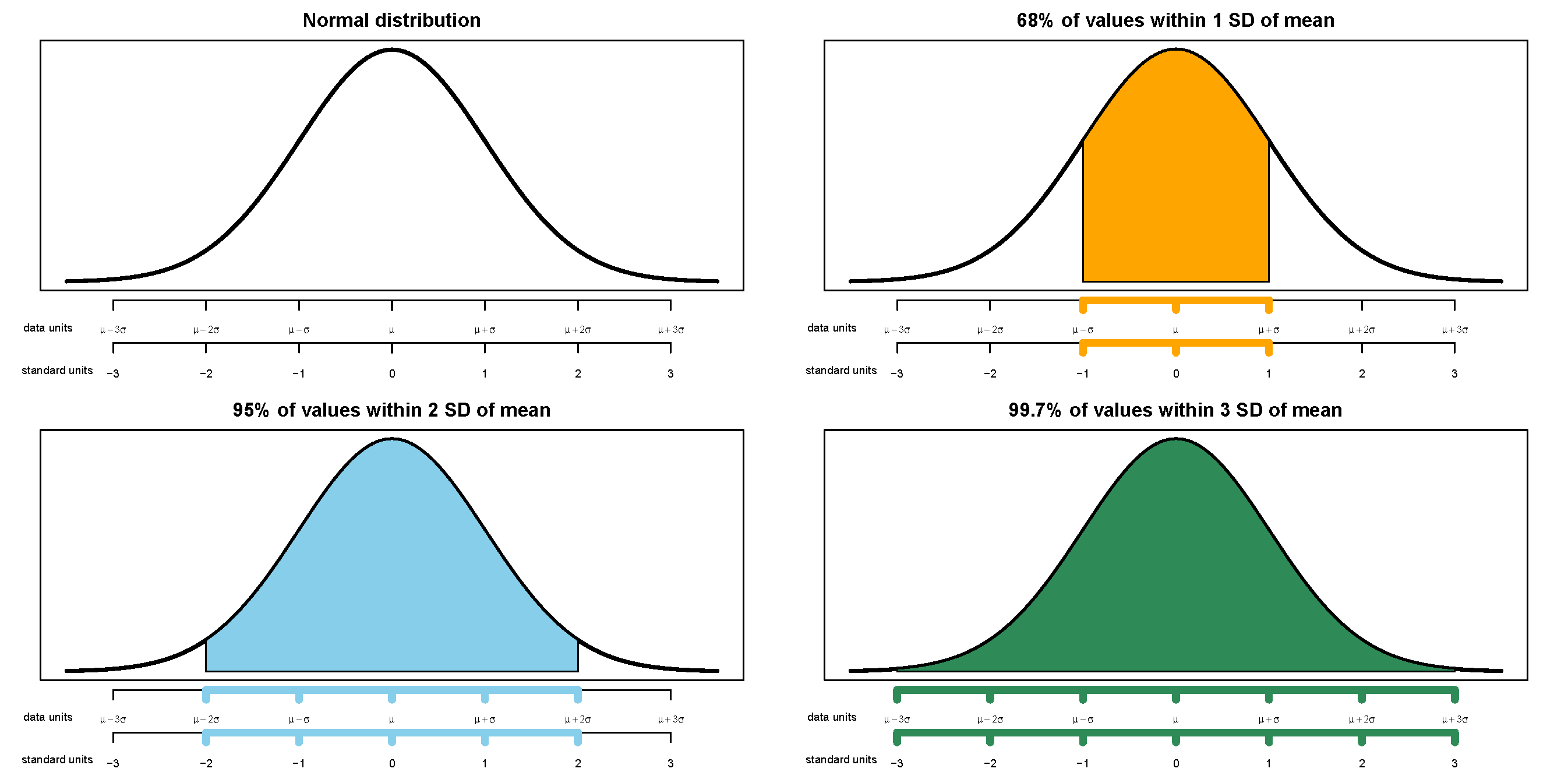
Figure 3.30: Illustration of the empirical rule for Normal distributions

Therefore the key to working with Normal distributions is to work in terms of standardized values. The “standard” Normal distribution is a Normal(0, 1) distribution, with a mean 0 and a standard deviation of 1. Notice how the empirical rule corresponds to the spinner in Figure 3.31.

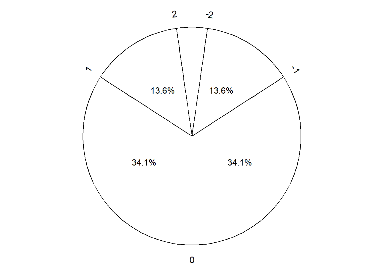
If a random variable follows a Normal distribution, a value of it can be simulated by spinning the standard Normal spinner in Figure 3.31 to determine how many standard deviations the value is away from the mean (above or below) and then converting to the measurement units of the variable.

We have only introduced a small part of the empirical rule in this section, corresponding to 1, 2, or 3 standard deviations away from the mean. We will cover Normal distributions and the empirical rule in much more detail later.

3.8.3 Exercises

Exercise 3.21 The latest series of collectible Lego Minifigures contains 3 different Minifigure prizes (labeled 1, 2, 3). Each package contains a single unknown prize. Suppose we only buy 3 packages and we consider as our sample space outcome the results of just these 3 packages (prize in package 1, prize in package 2, prize in package 3). For example, 323 (or (3, 2, 3)) represents prize 3 in the first package, prize 2 in the second package, prize 3 in the third package. Let $X$ be the number of distinct prizes obtained in these 3 packages. Let $Y$ be the number of these 3 packages that contain prize 1.

Explain how you could, in principle, conduct a simulation by hand and use the results to approximate
1. $\textrm{Var}(X)$
2. $\textrm{SD}(X)$
Write Symbulate code to conduct a simulation and approximate the values in part 1.
Compute the theoretical values of $\textrm{Var}(X)$ and $\textrm{SD}(X)$ and compare to the simulation results.

Exercise 3.22 Consider a continuous version of the dice rolling problem where instead of rolling two fair four-sided dice (which return values 1, 2, 3, 4) we spin twice a Uniform(1, 4) spinner (which returns any value in the continuous range between 1 and 4). Let $X$ be the sum of the two spins and let $Y$ be the larger of the two spins.

Use simulation to approximate the marginal distributions of $X$ and $Y$.
Which will have the larger standard deviation, $X$ or $Y$? Make a ballpark estimate the of the standard deviation of each.
Describe in words how you could use simulation to approximate
1. $\textrm{Var}(X)$ and $\textrm{SD}(X)$
2. $\textrm{E}(Y)$ and $\textrm{SD}(Y)$
Write Symbulate code to conduct a simulation to approximate the quantities in the previous part.

3.9 Measuring relationships: Covariance and correlation

Quantities like expected value, variance, and standard deviation summarize characteristics of the marginal distribution of a single random variable. When there are multiple random variables their joint distribution is of interest. Covariance and correlation each summarize in a single number a characteristic of the joint distribution of two random variables, namely, the degree to which they “co-deviate from the their respective means”.

3.9.1 Covariance

Consider the independent Uniform(0, 60) model of arrival times in the meeting problem from Section 3.4.1. Let $R$ and $Y$ be the two arrival times, and let $T=\min(R, Y)$ and $W=|R-Y|$ be the first arrival time and waiting time random variables, respectively. Our goal is to compute the covariance between $T$ and $W$.

We’ll illustrate the calculation using the simulation results from Table 3.3. The simulated $(T, W)$ pairs are displayed in Table 3.14. The mean of the 10 simulated values of $T$ is 22.6, and the mean of the 10 simulated values of $W$ is 20.7. We want to measure the degree to which $T$ and $W$ “co-deviate from the their respective means”. For each value of $T$ we find its deviation from the mean, and likewise for $W$; see the “T_deviation” and “W_deviation” columns of Table 3.14. Notice that we do care about the sign since we are interested in the relationship between $T$ and $W$, which involves questions like: if $T$ is above the mean, does $W$ tend to be above or below the mean? For each simulated $(T, W)$ pair, we now have a pair of deviations from the respective mean.

We want to measure the degree of co-deviation between $X$ and $Y$; one way to do this is to measure the interaction between the paired deviations by taking their product. See the “product_of_deviations” column of Table 3.14. Within each row, the value in the product column is the product of the values in the “T_devation” and “W_deviation” columns. The covariance is the average of the product of the deviations: sum the 10 values of the product and divide by 10 to get a covariance of -134.1. \[ \text{Covariance($X$, $Y$)} = \text{Average of} ((X - \text{Average of }X)(Y - \text{Average of }Y)) \]

Table 3.14: Calculation of covariance based on 10 simulated values

repetition	T	W	T_deviation	W_deviation	product_of_deviations
1	49.505	3.244	26.917	-17.458	-469.925
2	22.041	33.344	-0.547	12.643	-6.912
3	7.524	2.433	-15.064	-18.269	275.198
4	39.636	11.695	17.049	-9.007	-153.555
5	26.338	17.435	3.751	-3.267	-12.254
6	28.619	13.894	6.032	-6.808	-41.063
7	31.155	9.963	8.567	-10.739	-91.999
8	4.406	39.610	-18.181	18.908	-343.770
9	8.867	26.600	-13.721	5.898	-80.928
10	7.784	48.801	-14.803	28.099	-415.960
Sum	225.877	207.018	0.000	0.000	-1341.168
Average	22.588	20.702	0.000	0.000	-134.117

Why take the product of the deviations? For two random variables $X$ and $Y$:

If both $X$ and $Y$ values are far above the mean, the product of the deviations will be positive and large in magnitude
If both $X$ and $Y$ values are far below the mean, the product of the devations will be positive and large in magnitude
If the $X$ value is far above the mean but the $Y$ value is far below the mean, the product of the deviations will be negative and large in magnitude
If the $X$ value is far below the mean but the $Y$ value is far above the mean, the product of the deviations will be negative and large in magnitude
If the $X$ value is close to its mean, the product of the deviations will be close to 0 regardless of the $Y$ value
If the $Y$ value is close to its mean, the product of the deviations will be close to 0 regardless of the $X$ value

So the average of the products of the deviations gives insight to the overall relationship between $T$ and $W$; is the association:

positive: above average values of $X$ tend to be associated with above average values of $Y$, and below average values of $X$ tend to be associated with below average values of $Y$
negative: above average values of $X$ tend to be associated with below average values of $Y$, and below average values of $X$ tend to be associated with above average values of $Y$
zero: no overall positive or negative association between $X$ and $Y$.

Figure 3.32 visualizes the covariance calculation. The ten $(T, W)$ pairs from Table 3.14 are displayed in each plot. The green “+” represents the two means. Figure 3.32 (a) highlights the first row of Table 3.14. The horizontal orange segment represents the deviation of the $T$ value from the mean of the $T$ values, and the vertical blue segment represents the deviation of the $W$ value from the mean of the $W$ values. If we think of these deviations as the sides of the shaded rectangle, the area of the rectangle represents the magnitude of the product of the deviations. For this pair the product would be negative since the value of $T$ is above the mean but the value of $W$ is below the mean. Figure 3.32 (b) displays ten rectangles, one for each $(T, W)$ pair. The rectangles are shaded grey if the product of the deviations is negative, and yellow if positive. The covariance is the average of the ten areas, keeping in mind that the areas can represent either positive (yellow) or negative (gray) values. There is more gray area than yellow area, so the covariance is negative.

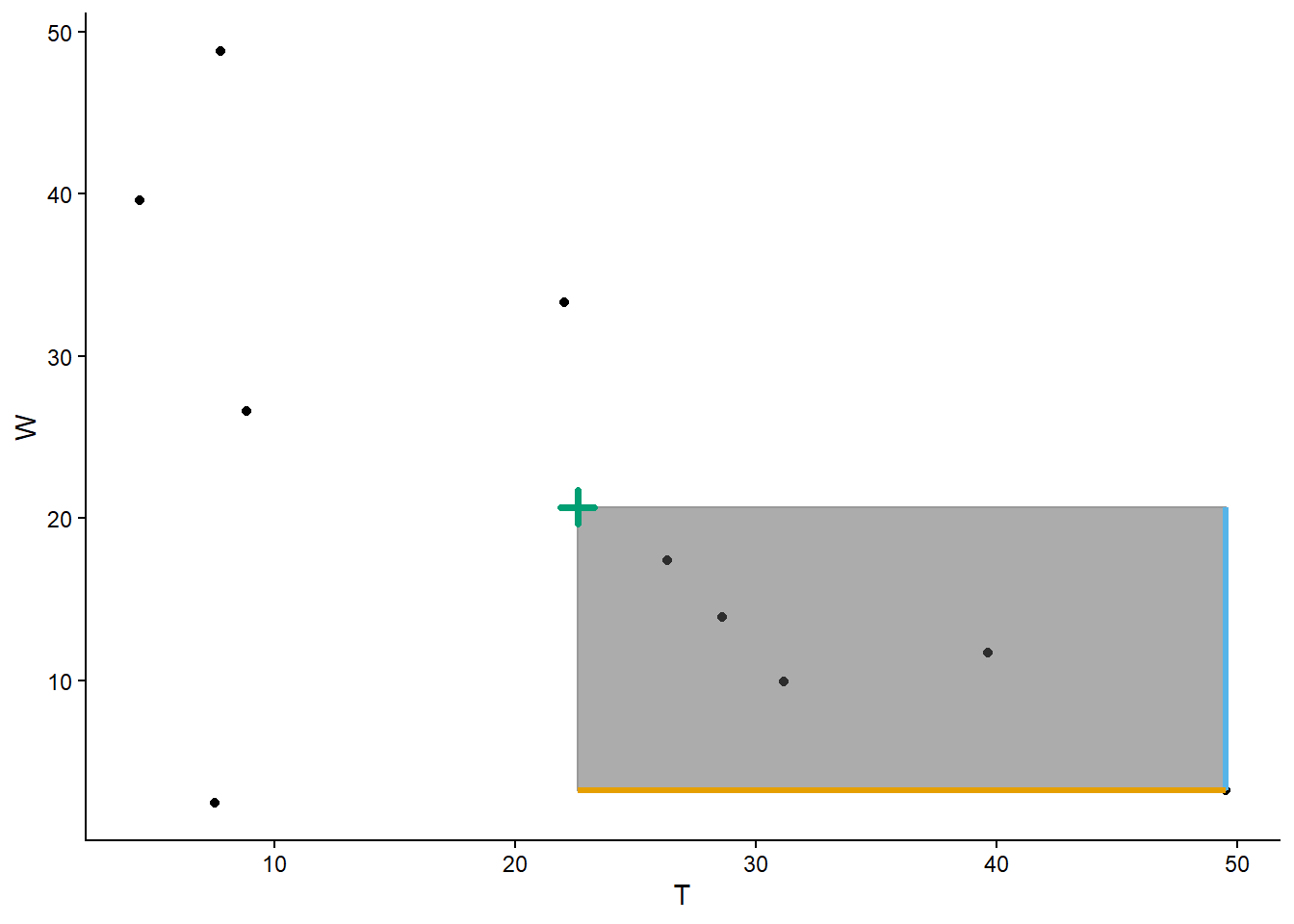
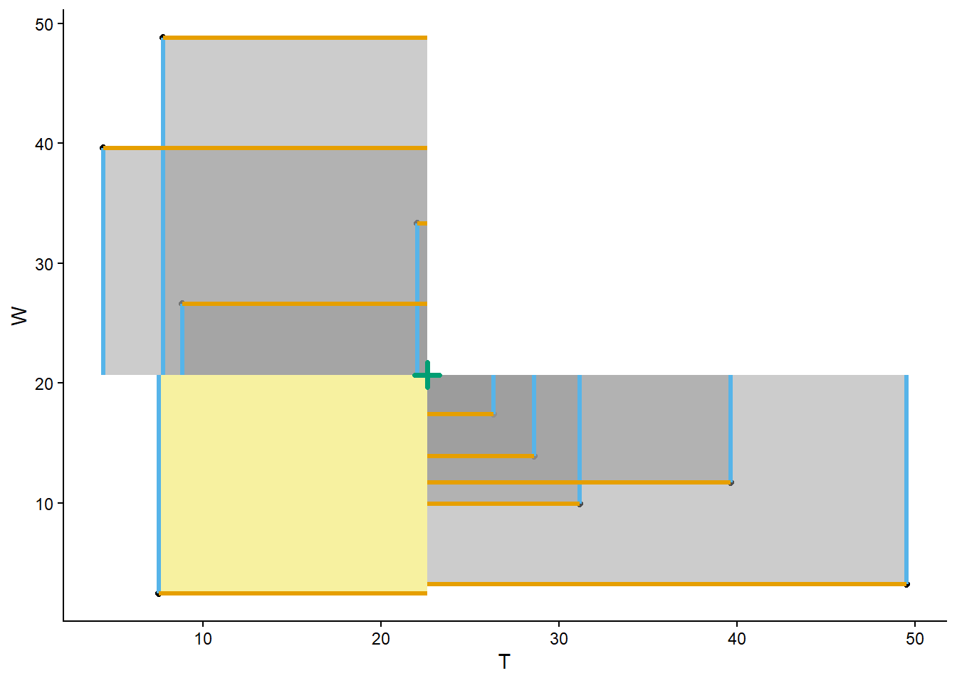
(a) A single point with its paired deviations and product rectangle

Table 3.14 and Figure 3.32 motivate the idea and calculation of covariance, but we’re really interested in what happens in the long run. We’ll start by simulating many $(T, W)$ pairs.

R, Y = RV(Uniform(0, 60) ** 2)

T = (R & Y).apply(min)

W = abs(R - Y)

meeting_sim = (R & Y & T & W).sim(10000)

t_and_w = meeting_sim[2, 3]

t_and_w

Index	Result
0	(21.333678740669104, 11.572778593030375)
1	(29.08298936668968, 1.4772167189851615)
2	(38.58468574670532, 16.662853627398647)
3	(7.755215577100216, 7.879322529642598)
4	(36.38391197683561, 7.702761765755163)
5	(16.94747418896801, 40.07014199132131)
6	(36.58802654389735, 8.002460291471053)
7	(40.07423800075149, 1.5375954717523257)
8	(31.43391163677623, 18.58407716464439)
...	...
9999	(8.125497025029205, 29.20230095039969)

t_and_w.plot()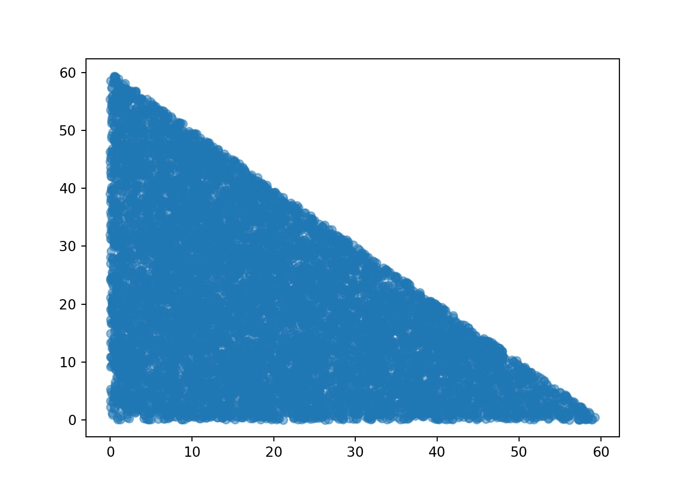

The simulated long run averages are (notice that calling mean returns the pair of averages)

t_and_w.mean()

(20.101705959948582, 19.86039753779092)

Now within each simulated $(t, w)$ pair, we subtract the mean of the $T$ values from $t$ and the mean of the $W$ values from $w$, We can do this subtraction in a “vectorized” way: the following code subtracts the first component of t_and_w.mean() (the average of the $T$) from the first component of each of the t_and_w values (the individual $t$ value), and similarly for the second.

t_and_w - t_and_w.mean()

Index	Result
0	(1.2319727807205219, -8.287618944760546)
1	(8.981283406741099, -18.38318081880576)
2	(18.482979786756736, -3.197543910392273)
3	(-12.346490382848366, -11.981075008148322)
4	(16.28220601688703, -12.157635772035757)
5	(-3.154231770980573, 20.209744453530387)
6	(16.486320583948768, -11.857937246319867)
7	(19.97253204080291, -18.322802066038594)
8	(11.332205676827648, -1.276320373146529)
...	...
9999	(-11.976208934919377, 9.341903412608769)

For each simulated pair, we now have a pair of deviations from the respective mean. To measure the interaction between these deviations, we take the product of the deviations within each pair. First, we split the paired deviations into two separate columns and then take the product within each row.

t_deviations = (t_and_w - t_and_w.mean())[0] # first column (Python 0)
w_deviations = (t_and_w - t_and_w.mean())[1] # second column (Python 1)

t_deviations * w_deviations

Index	Result
0	-10.210120956928726
1	-165.1045568510614
2	-59.100139463047476
3	147.92422736428816
4	-197.95313031856162
5	-63.74621803872397
6	-195.493754907176
7	-365.9527513412456
8	-14.463524978021876
...	...
9999	-111.88058711923895

Now we take the average of the products of the paired deviations.

(t_deviations * w_deviations).mean()

-98.72920358193242

This value is the covariance, which we could have arrived at more quickly by calling cov on the simulated $(T, W)$ pairs.

t_and_w.cov()

np.float64(-98.72920358193244)

The covariance between $T$ and $W$ is negative because the two variables have an overall negative association. The largest values of $T$ (near 60) are associated with the smallest values of $W$ (near 0) and vice versa. Since both people need to arrive in the 0 to 60 time interval, if the first person arrives very late then they won’t have to wait very long. Note that the association isn’t perfect; the smallest values of $T$ (near 0) are associated with the whole range of waiting times (from 0 to 60). But the overall tendency is a negative association.

Example 3.20 Now consider the arrival times $R$ and $Y$ of the two people in the meeting problem.

Explain in words in full detail how you could simulation to approximate the covariance between $R$ and $Y$. Assume that $R$ and $Y$ following the independent Uniform(0, 60) model of Section 3.4.1
For each of the following, explain if the covariance between $R$ and $Y$ will be positive, negative, or close to 0. Then use Symbulate to approximate the covariance.
- the independent Uniform(0, 60) model of Section 3.4.1
- the independent Normal(30, 10) model of Section 3.4.2
- the Bivariate Normal model of Section 3.4.3

Solution (click to expand)

Solution 3.20.

Spin the Uniform(0, 60) spinner twice to simulate an $(R, Y)$ pair. Repeat to simulate many $(R, Y)$ pairs. Compute the average of the simulated $R$ values and the deviations of the $R$ values from their average; likewise for $Y$. Now you have a pair of deviations for each repetition; compute the product of the paired deviations and then average the products to approximate the covariance between $R$ and $Y$. (The only difference for the other models in the next part would be how you simulate and $(R, Y)$ pair; once you have the pairs you would approximate the covariance using the same method.)
We basically assumed the covariance in definining the model for $R$ and $Y$
- $R$ and $Y$ are independent, so there will be no overall association and we expect the covariance to be near 0
- $R$ and $Y$ are independent, so there will be no overall association and we expect the covariance to be near 0. The pattern of variability of $(R, Y)$ would be different than in the previous part but there is still no relationship between $R$ and $Y$.
- We expect the covariance to be positive because we assumed that there was a positive association—they tend to arrive around the same time—when definiing the model.

# independent Uniform(0, 60)
meeting_sim[0, 1].cov()

np.float64(-1.0595951347503059)

# independent Normal(30, 10)

R, Y = RV(Normal(30, 10) ** 2)
(R & Y).sim(10000).cov()

np.float64(-0.5854995801936713)

# Bivariate Normal model

R, Y = RV(BivariateNormal(mean1 = 30, mean2 = 30, sd1 = 10, sd2 = 10, corr = 0.7))
(R & Y).sim(10000).cov()

np.float64(70.36460439821379)

The following definiton states our notion of covariance in expected value terms.

Definition 3.2 (Covariance between two random variables) The covariance between two random variables $X$ and $Y$ is \[ \textrm{Cov}(X, Y) = \textrm{E}((X-\textrm{E}(X))(Y-\textrm{E}(Y))) \]

Recall that an expected value is a long run average. Thefore we can interpret $\textrm{E}(\cdot)$ as “simulate many values of what’s inside $(\cdot)$ and average”. In this way \[ \textrm{E}((X-\textrm{E}(X))(Y-\textrm{E}(Y))) = \text{Long Run Average of} ((X - \text{Long Run Average of }X)(Y - \text{Long Run Average of }Y)) \] where the average is over many $(X, Y)$ pairs.

Unfortunately, the actual value of covariance is hard to interpret as it depends heavily on the measurement unit scale of the random variables. In the meeting problem, if $T$ and $W$ are both measured in minutes then the covariance is measured in minutes $\times$ minutes, e.g., -100 $\text{minutes}^2$. If we converted the $T$ values from minutes to seconds, then the value of covariance would change accordingly and would be measured in minutes $\times$ seconds, e.g., -6000 minutes $\times$ seconds. In another context, if the covariance between height (m) and weight (kg) is 0.3 $\text{m}\times\text{kg}$, then the covariance between height (cm) and weight (g) is 300,000 $\text{cm}\times\text{g}$.

But the sign of the covariance does have an intuitive meaning.

A positive covariance indicate an overall positive association: above average values of $X$ tend to be associated with above average values of $Y$
A negative covariance indicates am overall negative association: above average values of $X$ tend to be associated with below average values of $Y$
A covariance of zero indicates that the random variables are uncorrelated: there is no overall positive or negative association. But be careful: if $X$ and $Y$ are uncorrelated there can still be a relationship between $X$ and $Y$. We will see examples later that demonstrate that being uncorrelated does not necessarily imply that random variables are independent.

We discussed how variance has many nice theoretical properties, but standard deviation is easier to interpret. Similarly, covariance has many nice theoretical properties, but correlation is easier to interpret. We will introduce correlation in the next subsection.

Recall that for discrete random variables we can compute expected values as probability-weighted average values. We can compute covariances for discrete random variables in a similar way.

Example 3.21 In the dice rolling problem, let $X$ be the sum and $Y$ be the larger of the two rolls. The joint distribution of $X$ and $Y$ is represented³⁴ by Table 2.16. In Example 2.44 we computed $\textrm{E}(X) = 5$ and $\textrm{E}(Y) = 3.125$.

Will $\textrm{Cov}(X, Y)$ be positive, negative, or close to 0? Explain without computing.
Compute $\textrm{Cov}(X, Y)$.
Describe in detail how $\textrm{Cov}(X, Y)$ can be simulated via approximation
Write Symbulate code to approximate $\textrm{Cov}(X, Y)$ and compare to the values from part 2.

Solution (click to expand)

Solution 3.21.

The covariance will be positive. The smallest value of $Y$ only occurs with the smallest value of $X$, and when $Y$ is its largest value $X$ is above average.
For the pair (2, 1), which occurs with probability (1/16) the paired deviations are $(2-5, 1 - 3.125)$, the product is $(2-5)(1-3.125)$, and so the contribution to the probability-weighted average is $(2-5)(1-3.125)(1/16) = 0.3984$; see the first row of Table 3.13. We repeat for each possible $(X, Y)$ pair; see Table 3.13 for more detail. The covariance is the sum of the values in the last column, $\textrm{Cov}(X, Y) = 1.25$.
We have already discussed how to simulate $(X, Y)$ pairs in this content. To approximate the covariance
- Simulate many $(X, Y)$ pairs
- Compute the average of the simulated values of $X$ (to approximate $\textrm{E}(X)$), and likewise for $Y$
- From each simulated value of $X$ subtract the average, and likewise for $Y$
- Compute the product of the two deviations from the previous part for each simulated pair
- Average the products from the previous part to approximate the covariance
See below for the code, both the long way and using the cov shortcut. The simulation-based approximation is close to 1.25.

Table 3.15: Steps in computing the covariance of $X$ and $Y$ in Example 3.21.

$x$	$y$	$x - \textrm{E}(X)$	$y - \textrm{E}(Y)$	$(x - \textrm{E}(X))(y - \textrm{E}(Y))$	$\textrm{P}(X=x, Y=y)$	$(x - \textrm{E}(X))(y - \textrm{E}(Y))\textrm{P}(X=x,Y=y)$
2	1	-3	-2.125	6.375	0.0625	0.3984
3	2	-2	-1.125	2.250	0.1250	0.2812
4	2	-1	-1.125	1.125	0.0625	0.0703
4	3	-1	-0.125	0.125	0.1250	0.0156
5	3	0	-0.125	0.000	0.1250	0.0000
5	4	0	0.875	0.000	0.1250	0.0000
6	3	1	-0.125	-0.125	0.0625	-0.0078
6	4	1	0.875	0.875	0.1250	0.1094
7	4	2	0.875	1.750	0.1250	0.2188
8	4	3	0.875	2.625	0.0625	0.1641

P = BoxModel([1, 2, 3, 4], size = 2)

X = RV(P, sum)
Y = RV(P, max)

x_and_y = (X & Y).sim(10000)

x_and_y

Index	Result
0	(7, 4)
1	(2, 1)
2	(6, 4)
3	(5, 4)
4	(7, 4)
5	(4, 3)
6	(4, 3)
7	(6, 4)
8	(5, 4)
...	...
9999	(8, 4)

x_and_y.mean()

(5.0058, 3.1262)

x_and_y - x_and_y.mean()

Index	Result
0	(1.9942000000000002, 0.8738000000000001)
1	(-3.0058, -2.1262)
2	(0.9942000000000002, 0.8738000000000001)
3	(-0.005799999999999805, 0.8738000000000001)
4	(1.9942000000000002, 0.8738000000000001)
5	(-1.0057999999999998, -0.12619999999999987)
6	(-1.0057999999999998, -0.12619999999999987)
7	(0.9942000000000002, 0.8738000000000001)
8	(-0.005799999999999805, 0.8738000000000001)
...	...
9999	(2.9942, 0.8738000000000001)

x_deviations = (x_and_y - x_and_y.mean())[0] # first column (Python 0)
y_deviations = (x_and_y - x_and_y.mean())[1] # second column (Python 1)

x_deviations * y_deviations

Index	Result
0	1.7425319600000004
1	6.390931959999999
2	0.8687319600000003
3	-0.00506803999999983
4	1.7425319600000004
5	0.12693195999999984
6	0.12693195999999984
7	0.8687319600000003
8	-0.00506803999999983
...	...
9999	2.6163319600000006

(x_deviations * y_deviations).mean()

1.26146804

x_and_y.cov()

np.float64(1.2614680400000005)

Example 3.22 Continuing Example 3.21.

Compute $\textrm{E}(XY)$. (We’ll see why very soon.) Is it equal to $\textrm{E}(X)\textrm{E}(Y)$?
Describe in detail how $\textrm{E}(XY)$ can be approximated via simulation.
Compute $\textrm{E}(XY) - \textrm{E}(X)\textrm{E}(Y)$. What do you notice?

Solution (click to expand)

Solution 3.22.

If $X$ is 5 and $Y$ is 3, which occurs with probability 2/16, then the product $XY$ is (5)(3) = 15. To compute $\textrm{E}(XY)$ as a probability-weighted average value, multiply each possible of $XY$ by its probability and sum. \[ {\scriptsize (2)(1)(1/16)+(3)(2)(2/16)+(4)(2)(1/16)+(4)(3)(2/16)+(5)(3)(2/16)+(5)(4)(2/16)+(6)(3)(1/16)+(6)(4)(2/16)+(7)(4)(2/16)+(8)(4)(1/16) } \] $\textrm{E}(XY) = 16.875$. Notice this is not the same as $\textrm{E}(X)\textrm{E}(Y)=(5)(3.125) = 15.625$
We have already discussed how to simulate $(X, Y)$ pairs in this content. To approximate $\textrm{E}(XY)$
- Simulate many $(X, Y)$ pairs
- For each simulated $(X, Y)$ pair compute the product $XY$. For example, if $X$ is 5 and $Y$ is 3 then the product $XY$ is (5)(3)=15.
- Average the products from the previous part to approximate $\textrm{E}(XY)$ See the Symbulate code below.
$\textrm{E}(XY) - \textrm{E}(X)\textrm{E}(Y) = 16.875-(5)(3.125) = 1.25$, which is $\textrm{Cov}(X, Y)$.

x_and_y[0] * x_and_y[1]

Index	Result
0	28
1	2
2	24
3	20
4	28
5	12
6	12
7	24
8	20
...	...
9999	32

(x_and_y[0] * x_and_y[1]).mean()

16.9106

(x_and_y[0] * x_and_y[1]).mean() - x_and_y[0].mean() * x_and_y[1].mean()

1.2614680400000005

Example 3.22 illustrates an alternative formula for computing covariance. Definition 3.2 represents the concept of covariance. However, covariance is usually computed using the following equivalent but slightly simpler formula.

Lemma 3.2 \[ \textrm{Cov}(X, Y) = \textrm{E}(XY) - \textrm{E}(X)\textrm{E}(Y) \]

That is, the covariance of $X$ and $Y$ is the expected value of the product minus the product of the expected values.

We will see how to compute covariance for continuous random variables later. But Definition 3.2 and Lemma 3.2 apply for both discrete and continuous random variables. Furthermore, covariance can be approximated via simulation in the same way for discrete or continuous random variables: simulate many pairs of the random variables and compute the average of the products of the paired deviations from the respective means.

Example 3.23 Consider the probability space corresponding to two rolls of a fair four-sided die. Let $X$ be the sum of the two rolls, $Y$ the larger of the two rolls, $W$ the number of rolls equal to 4, and $Z$ the number of rolls equal to 1. Without doing any calculations, determine if the covariance between each of the following pairs of variables is positive, negative, or zero. Explain your reasoning conceptually.

$X$ and $W$
$X$ and $Z$
$X$ and $V$, where $V = W + Z$.
$W$ and $Z$. Hint: remember that there are two rolls.

Solution (click to expand)

Solution 3.23.

Positive. If $W$ is large (roll many 4s) then $X$ (sum) tends to be large.
Negative. If $Z$ is large (roll many 1s) then $X$ (sum) tends to be small.
Zero. Basically, the positive association between $X$ and $W$ cancels out with the negative association of $X$ and $Z$. $V$ is large when there are many 1s or many 4s, or some mixture of 1s and 4s. So knowing that W is large doesn’t really tell you anything about the sum.
Negative.
There is a fixed number of rolls. If you roll lots of 4s ($W$ is large) then there must be few rolls of 1s ($Z$ is small).

3.9.2 Correlation

The numerical value of the covariance depends on the measurement units of both variables, so interpreting it can be difficult. Covariance is a measure of joint association between two random variables that has many nice theoretical properties, but the correlation (coefficient) is often a more practical measure.

Recall that we can standardize a random variable to put in on a standard measurement scale in which values are measured in terms of standard deviations above or below the mean. It is useful to standardize random variables when measuring their co-deviation, measuring the deviations in standard deviation terms rather than measurement units. The correlation between two random variables is the covariance between the corresponding standardized random variables. Therefore, correlation is a standardized measure of the association between two random variables.

Definition 3.3 (Correlation between two random variables) The correlation (a.k.a. correlation coefficient) between two random variables $X$ and $Y$ is \[ \textrm{Corr}(X, Y) = \textrm{Cov}\left(\frac{X-\textrm{E}(X)}{\textrm{SD}(X)}\frac{Y-\textrm{E}(Y)}{\textrm{SD}(Y)}\right) \]

Returning to the $(T, W)$ example, we carry out the same process of computing the covariance, but first standardize each of the simulated values of $T$ by subtracting their mean and dividing by their standardization, and similarly for $W$. Then we compute the product for each pair of standardized values and average the products to get the correlation -0.619.

Table 3.16: Calculation of correlation based on 10 simulated values

repetition	T	W	T_standardized	W_standardized	product_of_standardized_values
1	49.5051230443642	3.24384813196957	1.8556242823391	-1.16810402389761	-2.16756219104242
2	22.0409069862217	33.3443601010367	-0.0376913487046098	0.845904484956141	-0.0318832809132752
3	7.52413982525468	2.4326638597995	-1.03844163845964	-1.2223799122306	1.26937019887689
4	39.6361792786047	11.6948688682169	1.17528352715253	-0.602650928322604	-0.708285708680737
5	26.3384757656604	17.4347750935704	0.258572492519595	-0.218596996291003	-0.0565231701882613
6	28.6194127053022	13.8940830063075	0.41581468549195	-0.455502733917882	-0.189404726044788
7	31.1545571219176	9.96297138277441	0.590581317853482	-0.718531225499212	-0.424351118074202
8	4.406319251284	39.6096999244764	-1.25337653465298	1.26511488670064	-1.58566531263075
9	8.86708207894117	26.6001215111464	-0.945862496382148	0.394651233192934	-0.373285800628161
10	7.78433695435524	48.8009335566312	-1.02050428715728	1.88009521530919	-1.91864522748692
Sum	225.876533011906	207.018325435929	1.52655665885959e-16	5.55111512312578e-17	-6.18623633681262
Average	22.5876533011906	20.7018325435929	1.52764086103208e-17	5.52943107967607e-18	-0.618623633681262
SD	14.5058835451554	14.9455733859826	1	1	NA

Now we repeat the same calculation for many (previously) simulated $(T, W)$ pairs.

t_and_w = meeting_sim[2, 3]

t_and_w

Index	Result
0	(21.333678740669104, 11.572778593030375)
1	(29.08298936668968, 1.4772167189851615)
2	(38.58468574670532, 16.662853627398647)
3	(7.755215577100216, 7.879322529642598)
4	(36.38391197683561, 7.702761765755163)
5	(16.94747418896801, 40.07014199132131)
6	(36.58802654389735, 8.002460291471053)
7	(40.07423800075149, 1.5375954717523257)
8	(31.43391163677623, 18.58407716464439)
...	...
9999	(8.125497025029205, 29.20230095039969)

Compute the means

t_and_w.mean()

(20.101705959948582, 19.86039753779092)

Compute the standard deviations

t_and_w.sd()

(14.009765869276556, 14.022716366805975)

We’ll use the standardize method to standardize the simulated values. Note that values are standardized using the respective means and standard deviations.

t_and_w.standardize()

Index	Result
0	(0.08793671444732995, -0.5910138041712569)
1	(0.641073055077749, -1.31095718817516)
2	(1.3192925534387372, -0.22802599915387106)
3	(-0.8812774244803222, -0.8544047169426784)
4	(1.1622040060351002, -0.866995769864877)
5	(-0.22514521658765257, 1.4412146637558827)
6	(1.1767734548728828, -0.8456234110524771)
7	(1.4256149765216786, -1.306651406671222)
8	(0.8088790192903365, -0.0910180552583795)
...	...
9999	(-0.854847186360425, 0.6661978441439889)

Now we compute the covariance of the standardized values to get the correlation.

t_and_w.standardize().cov()

np.float64(-0.5025538524109374)

We can also just call corr on the simulated $(T, W)$ pairs.

t_and_w.corr()

np.float64(-0.5025538524109379)

When standardizing, subtracting the means doesn’t change the scale of the possible pairs of values or how far away they are from their means; it merely shifts the center of the joint distribution. Dividing by the standard deviations does change the scale. It can be shown that correlation is the covariance divided by the product of the standard deviations.

Lemma 3.3 \[ \textrm{Corr}(X, Y) = \frac{\textrm{Cov}(X, Y)}{\textrm{SD}(X)\textrm{SD}(Y)} \]

The simulated values provide an example of this property.

t_and_w.cov() / (t_and_w.sd()[0] * (t_and_w.sd()[1]))

np.float64(-0.5025538524109376)

Definition 3.3 reflects the concept of correlation, but Lemma 3.3 is usually how we compute correlation. The hard work is in computing the covariance and the standard deviations; once we have those it’s just a matter of dividing to get the correlation.

Example 3.24 In the dice rolling problem, let $X$ be the sum and $Y$ be the larger of the two rolls.

Compute $\textrm{Corr}(X, Y)$.
Write Symbulate code to approximate $\textrm{Corr}(X, Y)$ and compare to the values from part 2.

Solution (click to expand)

Solution 3.24.

In Example 3.21 we computed $\textrm{Cov}(X, Y) = 1.25$, and in Example 3.17 we computed $\textrm{SD}(Y) = 0.927$. We just need to compute $\textrm{SD}(X)$. $\textrm{E}(X)=5$, $\textrm{E}(X^2) = 27.5$, $\textrm{Var}(X) = 2.5$, and $\textrm{SD}(X) = 1.581$. Therefore \[ \textrm{Corr}(X, Y) = \frac{\textrm{Cov}(X, Y)}{\textrm{SD}(X)\textrm{SD}(Y)} = \frac{1.25}{(1.581)(0.927)} = 0.853 \]
See the code below (we simulated x_and_y pairs previously).

x_and_y.sd()

(1.5869361549854413, 0.9345980740403467)

x_and_y.cov()

np.float64(1.2614680400000005)

x_and_y.corr()

np.float64(0.850534462722398)

A correlation coefficient has no units and is measured on a universal scale. Regardless of the original measurement units of the random variables $X$ and $Y$ \[ -1\le \textrm{Correlation}(X,Y)\le 1 \]

$\textrm{Correlation}(X,Y) = 1$ if and only if $Y=mX+b$ for some $m>0$
$\textrm{Correlation}(X,Y) = -1$ if and only if $Y=mX+b$ for some $m<0$

Therefore, correlation is a standardized measure of the strength of the linear association between two random variables. The closer the correlation is to 1 or $-1$, the closer the joint distribution of $(X, Y)$ pairs hugs a straight line, with positive or negative slope.

Because correlation is computed between standardized random variables, correlation is not affected by a linear rescaling of either variable. A value that is “one standard deviation above the mean” is “one standard deviation above the mean”, whether the variable measured in feet or inches or meters.

In some problems we are given the correlation and the standard deviations and we need to compute the covariance

\[ \textrm{Cov}(X, Y) = \textrm{Corr}(X, Y)\textrm{SD}(X)\textrm{SD}(Y) \]

3.9.3 Bivariate Normal distributions (briefly)

Just as Normal distributions are commonly assumed for marginal distributions of individual random variables, joint Normal distributions are often assumed for joint distributions of several random variables. We’ll focus “Bivariate Normal” distributions which describe a specific pattern of joint variability for two random variables.

Example 3.25 Donny Don’t has just completed a problem where it was assumed that SAT Math scores follow a Normal(500, 100) distribution. Now a follow up problem asks Donny how he could simulate a single (Math, Reading) pair of scores. Donny says: “That’s easy; just spin the Normal(500, 100) twice, once for Math and once for Reading.” Do you agree? Explain your reasoning.

Solution (click to expand)

Solution 3.25. You should not agree with Donny, for two reasons.

It’s possible that the distribution of SAT Math scores follow a different pattern than SAT Reading scores. So we might need one spinner to simulate a Math score, and a second spinner to simulate the Reading score. (In reality, SAT Math and Reading scores do follow pretty similar distributions. But it’s possible that they could follow different distributions.)
Furthermore, there is probably some relationship between scores. It is plausible that students who do well on one test tend to do well on the other. For example, students who score over 700 on Math are probably more likely to score above than below average on Reading. If we simulate a pair of scores by spinning one spinner for Math and a separate spinner for Reading, then there will be no relationship between the scores because the spins are physically independent.

In the previous problem, what we really need is a spinner that generates a pair of scores simultaneously to reflect their association. This is a little harder to visualize, but we could imagine spinning a “globe” with lines of latitude corresponding to SAT Math score and lines of longitutde to SAT Reading score. But this would not be a typical globe:

The lines of latitude would not be equally spaced, since SAT Math scores are not equally likely. (We have seen similar issues for one-dimensional Normal spinners.) Similarly for lines of longitude.
The scale of the lines of latitude would not necessarily match the scale of the lines of longitude, since Math and Reading scores could follow difference distributions. For example, the equator (average Math) might be 500 while the prime meridian (average Reading) might be 520.
The “lines” would be tilted or squiggled to reflect the relationship between the scores. For example, the region corresponding to Math scores near 700 and Reading scores near 700 would be larger than the region corresponding to Math scores near 700 but Reading scores near 200.

So we would like a model that

Simulates Math scores that follow a Normal distribution pattern, with some mean and some standard deviation.
Simulates Reading scores that follow a Normal distribution pattern, with possibly a different mean and standard deviation.
Reflects how strongly the scores are associated.

Such a model is called a “Bivariate Normal” distribution. There are five parameters: the two means, the two standard deviations, and the correlation which reflects the strength of the association between the two scores.

Recall that in Section 3.4.3 we assumed that Regina and Cady tend to arrive around the same time. One way to model pairs of values that have correlation is with a Bivariate Normal distribution, like in the following. We assumed a Bivariate Normal distribution for the $(R, Y)$ pairs, with mean (30, 30), standard deviation (10, 10) and correlation 0.7. (We could have assumed different means and standard deviations.)

R, Y = RV(BivariateNormal(mean1 = 30, sd1 = 10, mean2 = 30, sd2 = 10, corr = 0.7))

(R & Y).sim(1000).plot()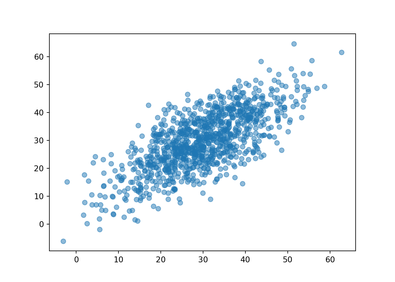

Now we see that the points tend to follow the $R = Y$ line, so that Regina and Cady tend to arrive near the same time.

Simulated values of a random variable with a Normal distribution follow a “bell-shaped” curve. Similarly, simulated pairs of values of two random variables with a Bivariate Normal distribution follow a “mound-shaped” or “fin-shaped” surface.

Figure 3.33 display a few Bivariate Normal distributions with different correlations. Notice how the correlation changes the shape of the distribution.

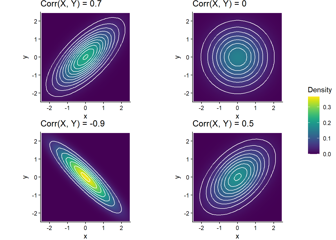
Figure 3.33: Bivariate Normal distributions

We will cover Bivariate Normal distributions in much more detail later.

3.9.4 Independent versus uncorrelated

The condition for independence of random variables is fairly strict. Random variables are independent only if the joint distribution is determined by the product of the marginal distributions for all values of the random variables. Otherwise, the random variables are not independent. However, you can imagine that there are different degrees of dependence.

We wish to measure degree of dependence in a single number. Unfortunately, there are many different ways two random variables can be related, and there is no single measure that works well in all cases.

The most commonly used measure of the degree of an association between two random variables is covariance, or its standardized counterpart, correlation.
While covariance does have many uses and nice properties, it does NOT measure whether two random variables are independent.

Example 3.26 Find $\textrm{Cov}(X,Y)$ in each of the following situations. Notice that the marginal distribution of $X$ is the same for each part, and similarly for $Y$.

$p_{X, Y}(x, y)$

$x$ \ $y$ -1 0 1 $p_X(x)$

0 1/6 1/6 1/6 1/2

1 1/6 1/6 1/6 1/2

$p_Y(y)$ 1/3 1/3 1/3
$p_{X, Y}(x, y)$

$x$ \ $y$ -1 0 1 $p_X(x)$

0 5/24 2/24 5/24 1/2

1 3/24 6/24 3/24 1/2

$p_Y(y)$ 1/3 1/3 1/3
In which of the previous parts are $X$ and $Y$ independent? Why?

Solution (click to expand)

Solution 3.26.

$\textrm{Cov}(X, Y) = \textrm{E}(XY) - \textrm{E}(X)\textrm{E}(Y) = \textrm{E}(XY)$ since $\textrm{E}(Y)=0$. $\textrm{E}(XY) = 0 + (1)(1)(1/6) + (1)(-1)(1/6) = 0$. So the covariance is 0.
Again, $\textrm{Cov}(X, Y) = \textrm{E}(XY)$ since $\textrm{E}(Y)=0$. $\textrm{E}(XY) = 0 + (1)(1)(3/24) + (1)(-1)(3/24) = 0$. So the covariance is 0.
$X$ and $Y$ are independent in part 1 because the joint distribution is the product of the marginal distributions. However, $X$ and $Y$ in part 2 are not independent even though the covariance is 0.

If $X$ and $Y$ are independent then $X$ and $Y$ are uncorrelated, that is, $\textrm{Cov}(X, Y) = 0$. However, the converse is not true in general: there are many situations in which $\textrm{Cov}(X, Y) = 0$ but $X$ and $Y$ are not independent. Independence means there is no probabilistic relationship between two random variables. Covariance only measures a particular kind of probabilistic relationship, namely: how closely do the $(X, Y)$ pairs tend to follow a single straight line with non-zero slope?

Correlation is most natural as a measure of association for Bivariate Normal distributions. If $X$ and $Y$ have a Bivariate Normal distribution and are uncorrelated, then $X$ and $Y$ are independent.

3.9.5 Exercises

Exercise 3.23 The latest series of collectible Lego Minifigures contains 3 different Minifigure prizes (labeled 1, 2, 3). Each package contains a single unknown prize. Suppose we only buy 3 packages and we consider as our sample space outcome the results of just these 3 packages (prize in package 1, prize in package 2, prize in package 3). For example, 323 (or (3, 2, 3)) represents prize 3 in the first package, prize 2 in the second package, prize 3 in the third package. Let $X$ be the number of distinct prizes obtained in these 3 packages. Let $Y$ be the number of these 3 packages that contain prize 1.

Explain how you could, in principle, conduct a simulation by hand and use the results to approximate $\textrm{Cov}(X, Y)$.
Write Symbulate code to conduct a simulation and approximate the covariance and correlation.
Compute $\textrm{Cov}(X, Y)$ and $\textrm{Corr}(X, Y)$.
Are $X$ and $Y$ independent? Explain your reasoning.

Exercise 3.24 Xavier and Yolanda are playing roulette. They both place bets on red on the same 3 spins of the roulette wheel before Xavier has to leave. (Remember, the probability that any bet on red on a single spin wins is 18/38.) After Xavier leaves, Yolanda places bets on red on 2 more spins of the wheel. Let $X$ be the number of bets that Xavier wins and let $Y$ be the number that Yolanda wins.

Find the marginal distribution of $X$.
Compute $\text{E}(X)$.
Compute $\textrm{Var}(X)$.
The joint distribution of $X$ and $Y$ is represented in the table below. Explain why $\textrm{P}(X=1, Y = 4) = 0$ and $\textrm{P}(X = 2, Y = 1) = 0$.
Compute $\textrm{P}(X = 2, Y = 3)$. (Yes, the table tells you it’s 0.1766, but show how this number can be computed based on the assumptions of the problem.)
Are $X$ and $Y$ independent? Justify your answer with an appropriate calculation.
Compute and interpret $\text{P}(X + Y = 4)$.
Make a table representing the marginal distribution of $X+Y$.
Use the table from the previous part to compute $\text{E}(X+Y)$, and verify that it is equal to $\text{E}(X)+\text{E}(Y)$. (It can be shown that $\textrm{E}(Y) = 5(18/38) = 2.37$)
Compute $\textrm{Cov}(X, Y)$. Interpret the sign of the covariance in context.
Compute $\textrm{Corr}(X, Y)$. (It can be shown that $\textrm{Var}(Y) = 5(18/38)(20/38) = 1.25$)

$x$, $y$	0	1	2	3	4	5
0	0.0404	0.0727	0.0327	0	0	0
1	0	0.109	0.1963	0.0883	0	0
2	0	0	0.0981	0.1766	0.0795	0
3	0	0	0	0.0294	0.053	0.0238

3.10 Conditioning

We can implement conditioning in simulations by only considering repetitions that satisfy the condition. Conditioning can be thought of as taking a subset of, or “filtering”, the simulation results.

3.10.1 Using simulation to approximate conditional probabilities

Conditional probabilities can be approximated using simulated relative frequencies in a similar way to unconditional probabilities, but the presence of conditioning requires more care.

Example 3.27 Recall Example 2.45. Consider simulating a randomly selected U.S. adult and determining whether or not the person is age 18-29 and whether or not they use Snapchat. Let $A$ be the event that the selected adult is age 18-29, $C$ be the event that the selected adult uses Snapchat, and $\textrm{P}$ correspond to randomly selecting an American adult. Suppose that $\textrm{P}(A) = 0.20$, $\textrm{P}(C) = 0.24$, and $\textrm{P}(A\cap C) = 0.13$.

Donny Don’t says, “we need two spinners to simulate this situation: One spinner with areas of 0.20 and 0.80 for age 18-29 or not, and another spinner with areas of 0.24 and 0.76 to represent uses Snapchat or not. Then spin each spinner once to simulate one repetition.” Do you agree? Explain.
How could you perform one repetition of the simulation using just a single spinner? (Hint: it needs 4 sectors.)
How could you perform a simulation, using the spinner in the previous part, to estimate $\textrm{P}(C | A)$?
What determines the order of magnitude of the the margin of error for your estimate in the previous part?
What is another method for performing the simulation and estimating $\textrm{P}(C |A)$ that has a smaller margin of error? What is the disadvantage of this method?

Solution (click to expand)

Solution 3.27.

Donny’s simulation assumes that age and Snapchat use are independent, but we know that younger people will be more likely to use Snapchat than older people. In general, you can not simulate pairs of events simply from the marginal probabilities of each.
You can construct a spinner for the possible occurrences of the pairs of events—both occur, $A$ occurs and $C$ does not, $C$ occurs and $A$ does not, neither occurs—and their joint probabilities. From the three given probabilities we can determine (see the interior cells in the two-way table in the solution to Example 2.45):
- age 18-29 and uses Snapchat: $\textrm{P}(A\cap C)= 0.13$
- age 18-29 and does not use Snapchat: $\textrm{P}(A\cap C^c)= 0.07$
- not age 18-29, and uses Snapchat: $\textrm{P}(A^c\cap C)= 0.11$
- not age 18-29, and does not use Snapchat: $\textrm{P}(A^c\cap C^c)= 0.69$ See the spinner in Figure 3.34.
The following method fixes the number of total spins, say 10000.
- Spin the joint spinner from the previous part once to simulate a (age, Snapchat) pair.
- Repeat a fixed number of times, say 10000.
- Discard the repetitions on which the person was not age 18-29, that is, the repetitions on which $A$ did not occur. You would expect to have around 2000 repetitions left.
- Among the remaining repetitions (on which $A$ occurred), count the number of repetitions on which $C$ also occurred. So for the roughly 2000 repetitions for which the person is age 18-29, count the repetitions on which the person also uses Snapchat; you would expect a count of around 1300.
- Estimate $\textrm{P}(C|A)$ by dividing the two previous counts to obtain a conditional relative frequency. \[ \textrm{P}(C | A)\approx \frac{\text{Number of repetitions on which both $A$ and $C$ occurred}}{\text{Number of repetitions on which $C$ occurred}} \]
Only those repetitions in which $A$ occurred are used to estimate $\textrm{P}(C|A)$. So the order of magnitude of the margin of error is determined by the number of repetitions on which $A$ occurs. This would be around 2000 repetitions for a margin of error of roughly $1/\sqrt{2000} = 0.022$, rather than 0.01 based on the original 10000 repetitions.
The previous method simulated a fixed number of repetitions first, and then discarded the ones that did not meet the condition $A$. We could instead discard repetitions that do not meet the condition as we go, and keep performing repetitions until we get a fixed number, say 10000, that do satisfy the condition $A$. In this way, the estimate $\textrm{P}(C |A)$ will be based on the fixed number of repetitions, say 10000, that satisfy event $A$. The disadvantage is increased computational burden; we will need to simulate and discard many repetitions in order to achieve the desired number that satisfy the condition. Roughly, we would need to simulate about 50000 repetitions in total to obtain 10000 repetitions that satisfy event $A$. The advantage is a more precise estimate of $\textrm{P}(C|A)$ than in the previous part.

The conditional probability of event $A$ given event $B$ can be approximated by simulating—according to the assumptions encoded in the probability measure $\textrm{P}$—the random phenomenon a large number of times and computing the relative frequency of $A$ among repetitions on which $B$ occurs.

\[ {\small \textrm{P}(A|B) \approx \frac{\text{number of repetitions on which $A$ and $B$ occur}}{\text{number of repetitions on which $B$ occurs}}, \quad \text{for a large number of repetitions simulated according to $\textrm{P}$} } \] When using simulation to approximate $\textrm{P}(A|B)$, we first use $B$ to determine which repetitions to keep, then we find the relative frequency of $A$.

Remember that the margin of error when approximating a probability based on a simulated relative frequency depends on the number of independently simulated repetitions used to calculate the relative frequency. When approximating $\textrm{P}(A|B)$ as above, the margin of error is determined by the number of independently simulated repetitions on which $B$ occurs.

There are two basic ways to use simulation³⁵ to approximate a conditional probability $\textrm{P}(A|B)$.

Simulate the random phenomenon for a set number of repetitions (say 10000), discard those repetitions on which $B$ does not occur, and compute the relative frequency of $A$ among the remaining repetitions (on which $B$ does occur).
- Disadvantage: the margin of error is based on only the number of repetitions used to compute the relative frequency. So if you perform 10000 repetitions but $B$ occurs only on 1000, then the margin of error for estimating $\textrm{P}(A|B)$ is roughly on the order of $1/\sqrt{1000} = 0.032$ (rather than $1/\sqrt{10000} = 0.01$). Especially if $\textrm{P}(B)$ is small, the margin of error could be large resulting in an imprecise estimate of $\textrm{P}(A|B)$.
- Advantage: not computationally intensive.
Simulate the random phenomenon until obtaining a certain number of repetitions (say 10000) on which $B$ occurs, discarding those repetitions on which $B$ does not occur as you go, and compute the relative frequency of $A$ among the remaining repetitions (on which $B$ does occur).
- Advantage: the margin of error will be based on the set number of repetitions on which $B$ occurs.
- Disadvantage: requires more time/computer power. Especially if $\textrm{P}(B)$ is small, it will require a large number of repetitions of the simulation to achieve the desired number of repetitions on which $B$ occurs. For example, if $\textrm{P}(B)=0.1$, then it will require roughly 100,000 repetitions in total to obtain 10,000 on which $B$ occurs.

3.10.2 Conditioning in Symbulate

In Symulate, filter can be used to extract repetitions that satisfy a condition. First we’ll simulate age and Snapchat use for 10000 hypothetical adults. Each ticket in the BoxModel has a (age, Snapchat) pair of labels, like the spinner in Figure 3.34.

P = BoxModel([('Age 18-29', 'Snapchat user'), ('Age 18-29', 'Not Snapchat user'), ('Not Age 18-29', 'Snapchat user'), ('Not Age 18-29', 'Not Snapchat user')],
             probs = [0.13, 0.07, 0.11, 0.69])

sim_all = P.sim(10000)

sim_all

Index	Result
0	('Age 18-29', 'Snapchat user')
1	('Not Age 18-29', 'Not Snapchat user')
2	('Not Age 18-29', 'Not Snapchat user')
3	('Not Age 18-29', 'Not Snapchat user')
4	('Age 18-29', 'Snapchat user')
5	('Not Age 18-29', 'Not Snapchat user')
6	('Not Age 18-29', 'Not Snapchat user')
7	('Not Age 18-29', 'Not Snapchat user')
8	('Age 18-29', 'Not Snapchat user')
...	...
9999	('Not Age 18-29', 'Not Snapchat user')

sim_all.tabulate()

Outcome	Frequency
('Age 18-29', 'Not Snapchat user')	697
('Age 18-29', 'Snapchat user')	1286
('Not Age 18-29', 'Not Snapchat user')	6900
('Not Age 18-29', 'Snapchat user')	1117
Total	10000

Now we’ll apply filter to retain only those age 18-29. The function is_Age18 takes as an input³⁶ a (age, Snapchat) pair and returns True if age 18-29 (and False otherwise). Applying filter(is_Age18) will only return results for which is_Age18 returns True.

def is_Age18(Age_Snapchat):
    return Age_Snapchat[0] == 'Age 18-29'
  
sim_given_Age18 = sim_all.filter(is_Age18)

sim_given_Age18

Index	Result
0	('Age 18-29', 'Snapchat user')
1	('Age 18-29', 'Snapchat user')
2	('Age 18-29', 'Not Snapchat user')
3	('Age 18-29', 'Not Snapchat user')
4	('Age 18-29', 'Snapchat user')
5	('Age 18-29', 'Snapchat user')
6	('Age 18-29', 'Not Snapchat user')
7	('Age 18-29', 'Snapchat user')
8	('Age 18-29', 'Not Snapchat user')
...	...
1982	('Age 18-29', 'Snapchat user')

sim_given_Age18.tabulate()

Outcome	Frequency
('Age 18-29', 'Not Snapchat user')	697
('Age 18-29', 'Snapchat user')	1286
Total	1983

Conditional relative frequencies are computed based only on repetitions which satisfy the event being conditioned on.

sim_given_Age18.tabulate(normalize = True)

Outcome	Relative Frequency
('Age 18-29', 'Not Snapchat user')	0.35148764498234997
('Age 18-29', 'Snapchat user')	0.64851235501765
Total	1.0

Based on these results, we would estimate $\textrm{P}(C |A)$ to be around the true value of 0.65 with a margin of error of roughly $1/\sqrt{2000} = 0.022$.

In Symbulate, the “given” symbol | applies the second method to simulate a fixed number of repetitions that satisfy the event being conditioned on. Be careful when using | when conditioning on an event with small probability. In particular, be careful when conditioning on the value of a continuous random variable (which we’ll discuss in more detail soon).

Below we use RV syntax to carry out the simulation and conditioning³⁷. Technically, a random variable always returns a number, but RV in Symbulate does allow for non-numerical outputs. In most situations, we will usually deal with true random variables, and the code syntax below will be more natural.

The following code simulates (Age, Snapchat) pairs until 10000 adults age 18-29 are obtained.

Age, Snapchat = RV(P)

sim_given_Age18 = ( (Age & Snapchat) | (Age == 'Age 18-29') ).sim(10000)

sim_given_Age18

Index	Result
0	(Age 18-29, Not Snapchat user)
1	(Age 18-29, Not Snapchat user)
2	(Age 18-29, Not Snapchat user)
3	(Age 18-29, Not Snapchat user)
4	(Age 18-29, Snapchat user)
5	(Age 18-29, Snapchat user)
6	(Age 18-29, Snapchat user)
7	(Age 18-29, Not Snapchat user)
8	(Age 18-29, Not Snapchat user)
...	...
9999	(Age 18-29, Snapchat user)

sim_given_Age18.tabulate()

Value	Frequency
(Age 18-29, Not Snapchat user)	3499
(Age 18-29, Snapchat user)	6501
Total	10000

Since all 10000 simulated pairs satisfy the event being conditioned on (age 18-29), they are all included in the computation of the conditional relative frequencies.

sim_given_Age18.tabulate(normalize = True)

Value	Relative Frequency
(Age 18-29, Not Snapchat user)	0.3499
(Age 18-29, Snapchat user)	0.6501
Total	1.0

Based on these results, we would estimate $\textrm{P}(C |A)$ to be around the true value of 0.65 with a margin of error of roughly $1/\sqrt{10000} = 0.01$. We have obtained a more precise estimate, but the simulation takes longer to run.

3.10.3 Using conditional probabilities to simulate

In Example 3.27 we directly simulated pairs of events using joint probabilities, and used the results to approximate conditional probabilities. But in many problems conditional probabilities are provided or can be determined directly.

Example 3.28 Recall Example 2.46. Suppose that

65% of American adults age 18-29 use Snapchat
24% of American adults age 30-49 use Snapchat
12% of American adults age 50-64 use Snapchat
2% of American adults age 65+ use Snapchat

Also suppose that

20% of American adults are age 18-29
33% of American adults are age 30-49
25% of American adults are age 50-64
22% of American adults are age 65+

Consider simulating a randomly selected U.S. adult and determining the person’s age group and whether or not they use Snapchat. How could you perform one repetition of the simulation using spinners based solely on the percentages provided above, without first constructing a two-way table or finding $\textrm{P}(A_1\cap C)$, etc? (Hint: you’ll need a few spinners, but you might not spin them all in a single repetition.)

Solution (click to expand)

Solution 3.28. It’s a two-stage simulation: first spin a spinner to determine age group, then given the result spin an appropriate spinner to determine Snapchat use. There will be 4 spinners for Snapchat use, but only 1 will be spun—along with the age spinner—in any single repetition. See Figure 3.35.

“Age” spinner: Areas of 0.20, 0.33, 0.25, 0.22 corresponding to, respectively, 18-29, 30-49, 50-64. 65+. Spin this to determine age group.
“Snapchat” spinners—only one of the following will be spun in a single repetition:
- Snapchat given age 18-29: areas of 0.65 and 0.35 corresponding to, respectively, uses Snapchat and does not use Snapchat. If the result of the “age” spinner is 18-29, spin this spinner to determine whether or not the person uses Snapchat.
- Snapchat given age 30-49: areas of 0.24 and 0.76 corresponding to, respectively, uses Snapchat and does not use Snapchat. If the result of the “age” spinner is 30-49, spin this spinner to determine whether or not the person uses Snapchat.
- Snapchat given age 50-64: areas of 0.12 and 0.88 corresponding to, respectively, uses Snapchat and does not use Snapchat. If the result of the “age” spinner is 50-64, spin this spinner to determine whether or not the person uses Snapchat.
- Snapchat given age 65+: areas of 0.02 and 0.98 corresponding to, respectively, uses Snapchat and does not use Snapchat. If the result of the “age” spinner is 65+, spin this spinner to determine whether or not the person uses Snapchat.

Figure 3.35: Spinners corresponding to Example 3.28. The spinner in the top row is spun first to simulate age group, then the corresponding spinner in the bottom row is spun to determine Snapchat use.

A two-stage simulation like the one above basically implements the multiplication rule, joint = conditional $\times$ marginal. We first simulate age based on marginal probabilities, then use conditional probabilities to simulate Snapchat use, resulting in (age, Snapchat) pairs with the appropriate joint relationship.

In Symbulate, we can code the scenario in Example 3.28 by defining a custom probability space. An outcome is a (Age, Snapchat) pair. Each of the 5 spinners corresponds to a BoxModel. We define a function that defines how to simulate one repetition in two stages, using the draw method³⁸. Then we use that function to define a custom ProbabilitySpace.

def Age_Snapchat_sim():
    Age = BoxModel(['18-29', '30-49', '50-64', '65+'], probs = [0.20, 0.33, 0.25, 0.22]).draw()
    if Age == '18-29':
        Snapchat = BoxModel(['Use', 'NotUse'], probs = [0.65, 0.35]).draw()
    if Age == '30-49':
        Snapchat = BoxModel(['Use', 'NotUse'], probs = [0.24, 0.76]).draw()
    if Age == '50-64':
        Snapchat = BoxModel(['Use', 'NotUse'], probs = [0.12, 0.88]).draw()
    if Age == '65+':
        Snapchat = BoxModel(['Use', 'NotUse'], probs = [0.02, 0.98]).draw()
    return Age, Snapchat
    
P = ProbabilitySpace(Age_Snapchat_sim)
P.sim(10)

Index	Result
0	('18-29', 'NotUse')
1	('30-49', 'Use')
2	('30-49', 'NotUse')
3	('18-29', 'Use')
4	('65+', 'NotUse')
5	('18-29', 'NotUse')
6	('50-64', 'NotUse')
7	('18-29', 'Use')
8	('18-29', 'Use')
...	...
9	('50-64', 'NotUse')

Once we have simulated pairs, we can proceed as in Section 3.10.1. For example, the following approximates conditional probabilities of age group given that the adult uses Snapchat, based on 10000 repetitions which satisfy the condition; compare to part 7 of Example 2.46.

Age, Snapchat = RV(P)

sim_given_Snapchat = ( Age | (Snapchat == 'Use') ).sim(10000)

sim_given_Snapchat.tabulate(normalize = True)

Value	Relative Frequency
18-29	0.5379
30-49	0.3235
50-64	0.1221
65+	0.0165
Total	1.0

3.10.4 Conditioning on values of random variables

If $X$ is a discrete random variable, we can condition on it equalling the value $x$ by conditioning on the event $\{X = x\}$.

Example 3.29 We’ll continue with the dice rolling example: roll two fair four-sided dice and let $X$ be the sum and $Y$ the larger of the rolls. For each of the following, describe how to approximate the probability based on 10000 repetitions of a tactile simulation (in principle).

$\textrm{P}(X = 6 | Y = 4)$.
$\textrm{P}(Y = 4 | X = 6)$.

Solution (click to expand)

Solution 3.29. We have already seen how to simulate $(X, Y)$ pairs.

Simulate an $(X, Y)$ pair. If $Y=4$ keep the pair, otherwise discard it. Continue until 10000 $(X, Y)$ pairs with $Y=4$ are obtained. Count the number of pairs for which $X=6$ and divide by 10000 to approximate $\textrm{P}(X = 6 | Y = 4)$, with a margin of error of 0.01.
Simulate an $(X, Y)$ pair. If $X=6$ keep the pair, otherwise discard it. Continue until 10000 $(X, Y)$ pairs with $X=6$ are obtained. Count the number of pairs for which $Y=4$ and divide by 10000 to approximate $\textrm{P}(Y = 4 | X = 6)$, with a margin of error of 0.01.

To approximate a conditional probability of an event involving a random variable $X$ given the value of a random variable $Y$, we first need to simulate $(X, Y)$ pairs. The variable being conditioned on ($Y$ here) determines which pairs to keep, and the other variable determines what to find the relative frequency of.

Here is some code for conditioning on $\{Y = 4\}$.

P = DiscreteUniform(1, 4) ** 2

X = RV(P, sum)
Y = RV(P, max)

( (X & Y) | (Y == 4) ).sim(10)

Index	Result
0	(7, 4)
1	(8, 4)
2	(8, 4)
3	(5, 4)
4	(7, 4)
5	(5, 4)
6	(5, 4)
7	(7, 4)
8	(5, 4)
...	...
9	(8, 4)

(X | (Y == 4) ).sim(10000).tabulate()

Value	Frequency
5	2846
6	2922
7	2814
8	1418
Total	10000

(X | (Y == 4) ).sim(10000).tabulate(normalize = True)

Value	Relative Frequency
5	0.2883
6	0.2812
7	0.2866
8	0.1439
Total	1.0

Below we simulate values of $X$ given $Y=y$ for each of the values $y = 2, 3, 4$. (We omit conditioning on $Y=1$ since then $X = 2$ with probability 1.) Each of the three simulations below approximates a separate conditional distribution of $X$ values.


x_given_Y_eq4 = (X | (Y == 4) ).sim(10000)

x_given_Y_eq3 = (X | (Y == 3) ).sim(10000)

x_given_Y_eq2 = (X | (Y == 2) ).sim(10000)

We plot the three distributions on a single plot to compare how the distribution of $X$ changes depending on the given value of $Y$.

x_given_Y_eq4.plot()
x_given_Y_eq3.plot(jitter = True) # shifts the spikes a little
x_given_Y_eq2.plot(jitter = True) # so they don't overlap

Extra care is required when conditioning on the value of a continuous random variable. We’ll consider the Bivariate Normal model of the meeting problem from Section 3.4.

Example 3.30 Suppose we want to approximate the conditional probability that Cady arrives first given that Regina arrives at 12:40.

Donny Don’t writes the Symbulate code below to approximate this probability. What do you think will happen when Donny runs his code?
Can you think of how to fix Donny’s code? (Hint: when we say “Regina arrives at 12:40”, what do we really mean?)

# Donny's code - don't try to run this!
R, Y = RV(BivariateNormal(mean1 = 30, sd1 = 10, mean2 = 30, sd2 = 10, corr = 0.7))

y_given_Req40 = (Y | (R == 40) ).sim(10000)

y_given_Req40.count_lt(40) / 10000

Solution (click to expand)

Solution 3.30.

Donny’s code will run forever! Using .sim(10000) with conditioning via | will continue the simulation until obtaining 10000 repetitions that satisfy the condition. Remember, $R$ is a continuous random variable, so $\textrm{P}(R = 40)=\textrm{P}(R = 40.00000000000000000\ldots) = 0$. The simulation will never return a single $(R, Y)$ pair with $Y$ equal to $40.0000000000000\ldots$, let alone 10000 of them.
“Regina arrives at 12:40” doesn’t really mean $R$ “is equal to 40” but rather $R$ “is close enough to 40”, where “close enough” depends on the context. Here, rounding to the nearest minute seems reasonable, in which case “Regina arrives at 12:40” really means “Regina arrives within 0.5 minutes (30 seconds) of 12:40”. So we want to condition on the event $\{40 - 0.5 < R < 40 + 0.5\}=\{|R - 40|<0.5\}$ rather than $\{R = 40\}$. See the code below, where we condition on the event (abs(R - 40) < 0.5). Aside from the conditioning event, Donny’s code is fine, but note that we have changed the number of repetitions from 10000 to 1000; see the discussion below.

R, Y = RV(BivariateNormal(mean1 = 30, sd1 = 10, mean2 = 30, sd2 = 10, corr = 0.7))

y_given_Req40 = (Y | (abs(R - 40) < 0.5) ).sim(1000)

y_given_Req40.count_lt(40) / 1000

0.654

Warning

Be careful when conditioning on the value of a continuous random variable. Remember that the probability that a continuous random variable is equal to a particular value is 0. Mathematically, when we condition on $\{X=x\}$ we are really conditioning on $\{|X-x|<\epsilon\}$—the event that the random variable $X$ is within $\epsilon$ of the value $x$—and seeing what happens in the idealized limit when $\epsilon$ approaches 0. Practically, $\epsilon$ represents the degree of precision which determines “close enough” in the problem context, e.g., $\epsilon=0.01$ if “within 0.01” is close enough. When conditioning on a continuous random variable $X$ in a simulation, never condition on $\{X=x\}$; rather, condition on $\{|X-x|<\epsilon\}$ where $\epsilon$ represents a suitable degree of precision. What counts as “suitable” depends on the context and the scale of the $X$ variable. For example, if our variable is household income (U.S. dollars) and we’re conditioning on household income “equal to” 100,000 dollars, then $\epsilon$ of 1000 dollars might be reasonable.

The event $\{|X-x|<\epsilon\}$ will have non-zero probability, but the probability might be small. Conditioning on low probability events introduces some computational challenges. Remember that the margin of error in using a relative frequency to approximate a probability is based on the number of independently simulated repetitions used to compute the relative frequency. When approximating a conditional probability with a conditional relative frequency, the margin of error is based only on the number of repetitions that satisfy the condition. Naively discarding repetitions that do not satisfy the condition can be horribly inefficient. For example, when conditioning on an event with probability 0.01 we would need to run about 1,000,000 repetitions to achieve 10,000 that satisfy the condition. There are more sophisticated and efficient methods (e.g., “Markov chain Monte Carlo (MCMC)” methods), but they are beyond the scope of this book. When conditioning on the value of a continuous random variable with | in Symbulate, be aware that you might need to change either the number of repetitions (but try not to go below 1000) or the degree of precision $\epsilon$ in order for the simulation to run in a reasonable amount of time.

In the Bivariate Normal model of the meeting problem the event $\{|R - 40| < 0.5\}$ has probability 0.04. Running (Y | (abs(R - 40) < 0.5) ).sim(1000) requires about 25000 repetitions in the background to achieve the 1000 the satisfy the condition. The margin of error for approximating conditional probabilities is roughly $1/\sqrt{1000} = 0.03$.

R, Y = RV(BivariateNormal(mean1 = 30, sd1 = 10, mean2 = 30, sd2 = 10, corr = 0.7))

( (R & Y) | (abs(R - 40) < 0.5) ).sim(10)

Index	Result
0	(39.696217935960306, 29.021463953892873)
1	(39.79766640272294, 33.47739689498418)
2	(39.82512574204207, 48.90927447122735)
3	(40.13011281775823, 40.02794636044875)
4	(40.441165065334076, 26.089893918129583)
5	(39.586728787258075, 35.12219885340394)
6	(40.04852404537298, 40.63930821498815)
7	(40.340031933692686, 34.07977035160372)
8	(40.29523559218278, 28.977271424889093)
...	...
9	(39.54185394658454, 26.89454554764432)

3.10.5 Conditional averages

TBA

3.10.6 Exercises

Exercise 3.25 The latest series of collectible Lego Minifigures contains 3 different Minifigure prizes (labeled 1, 2, 3). Each package contains a single unknown prize. Suppose we only buy 3 packages and we consider as our sample space outcome the results of just these 3 packages (prize in package 1, prize in package 2, prize in package 3). For example, 323 (or (3, 2, 3)) represents prize 3 in the first package, prize 2 in the second package, prize 3 in the third package. Let $X$ be the number of distinct prizes obtained in these 3 packages. Let $Y$ be the number of these 3 packages that contain prize 1.

Explain how you could, in principle, conduct a simulation by hand and use the results to approximate
1. $\textrm{P}(Y = 0 | X = 1)$
2. The conditional distribution of $Y$ given $X=1$
3. $\textrm{P}(X = 1 | Y = 0)$
4. The conditional distribution of $X$ given $Y=0$
Write Symbulate code to conduct a simulation and approximate the values in part 1. Each simulation should be based on 10000 repetitions that satisfy the conditioning event.

Exercise 3.26 Write Symbulate code to conduct the simulation in Exercise 3.4. Use conditioning to discard any repetitions where the dart lands off the board. Use the simulation results to approximate:

The marginal distribution of $R$ (via plot)
$\textrm{P}(R < 1)$
$\textrm{P}(R > 11)$
$\textrm{E}(R)$
$\textrm{SD}(R)$.

Exercise 3.27 Consider a continuous version of the dice rolling problem where instead of rolling two fair four-sided dice (which return values 1, 2, 3, 4) we spin twice a Uniform(1, 4) spinner (which returns any value in the continuous range between 1 and 4). Let $X$ be the sum of the two spins and let $Y$ be the larger of the two spins.

Describe in words how you could use simulation to approximate
1. $\textrm{P}(Y < 2.7 | X = 3.5)$
2. The conditional distribution of $Y$ given $X = 3.5$
Write Symbulate code to conduct a simulation to approximate the quantities from the previous part.

Hint: be careful! What do we really mean by conditioning on $X = 3.5$?

3.11 Independence

For independent events, the multiplication rule simplifies

\[\begin{align*} \text{If $A$ and $B$ are independent then } && \textrm{P}(A \cap B) & = \textrm{P}(A)\textrm{P}(B)\\ \text{If independent then } && \text{Joint} & = \text{Product of Marginals} \end{align*}\]

Similarly, the joint distribution of independent random variables is this product of their marginal distributions. For this reason, independence is represented by the product * syntax in Symbulate.

For example, in the meeting problem, if Regina’s arrival follows a Uniform(0, 60) model, Cady’s follows a Normal(30, 10) model, and they arrive independently of each other, we can simulate pairs of arrivals as follows; note the use of *.

P = Uniform(0, 60) * Normal(30, 10)
P.sim(5)

Index	Result
0	(53.58860978904647, 51.330985933234594)
1	(20.796385530547866, 17.063118545209722)
2	(54.87878043505233, 23.55243324151116)
3	(54.53010802402967, 5.411783602714628)
4	(49.70559012140185, 22.421491538455673)

We can think of * as “spin each spinner independently”, but what * really does is create a joint probability space as the product of two marginal probability spaces.

Warning

Be careful: * plays different roles for probability spaces and named distributions (like Uniform, Normal) than it does for random variables. Using * with probability spaces indicates that the spaces are independent. Likewise, using * with distributions of random variables, as in X, Y = RV(Distribution_X * Distribution_Y), indicates that the random variables are independent since their joint distribution is the product of their marginal distributions. In contrast, using * directly on random variables, as in X * Y, literally means multiplication. (Section 3.15 has further discussion on the difference between a random variable and its distribution.)

Note the two uses of * in the code below. In the P = ... line, * means that the two components of the pair will be simulated independently (e.g., “spin the Uniform(0, 60) spinner then spin the Normal(30, 10) spinner”), resulting in random variables R (first component) and Y (second component) that are independent. In (R * Y), * means multiply the values of R and Y.

P = Uniform(0, 60) * Normal(30, 10)
R, Y = RV(P)

(R & Y & (R * Y) ).sim(5)

Index	Result
0	(39.25570090222384, 20.264451338103925, 795.4952406762774)
1	(40.980446638854396, 24.064641797170033, 986.1797690520717)
2	(54.7746130593508, 16.479798417834555, 902.6745816329892)
3	(18.930492145303898, 25.121425519590865, 475.56094847745175)
4	(27.173248635804676, 29.389142413870534, 798.5984740051769)

We could have also coded the following, which we interpret as defining random variables R and Y whose joint distribution is the product of their marginal distributions, Uniform(0, 60) for R and Normal(30, 10) for Y, and thus R and Y are independent.

R, Y = RV(Uniform(0, 60) * Normal(30, 10))

(R & Y & (R * Y) ).sim(5)

Index	Result
0	(32.010521841803076, 35.57205404485328, 1138.6800129605754)
1	(41.79316026473473, 23.19780374105788, 969.5095295398949)
2	(26.065182376890437, 26.592139208953636, 693.1289582730356)
3	(59.13146318697971, 29.860590174498455, 1765.7003886448433)
4	(20.384036497977593, 16.19374454631192, 330.0938798709478)

Example 3.31 Donny Don’t writes the following code to simulate $X$ and $Y$ from Example 2.68, but it returns an error. Can you explain why? Think about it first, but if you need a hint, run the code to see the error. How could you fix the code so it runs properly.

X = RV(BoxModel([2, 3, 4, 5, 6, 7, 8], probs = [1/16, 2/16, 3/16, 4/16, 3/16, 2/16, 1/16]))
Y = RV(BoxModel([1, 2, 3, 4], probs = [1/16, 3/16, 5/16, 7/16]))

(X & Y).sim(10)

Solution (click to expand)

Solution 3.31. Donny’s code defines the correct marginal distributions for $X$ and $Y$, but to simulate $X, Y$ pairs we need to know their joint distribution. Recall the moral of Example 2.68 and the discussion following it: marginal distributions alone are not enough to determine the joint distribution.

The error message is “Events must be defined on same probability space”, which in this case really should be “random variables must be defined on same probability space”, but even that is maybe not the most informative message. The idea is that we have not provided enough information to determine how to pair $X$ and $Y$ values when running the simulation. If the random variables were defined on the same probability space, the probaility space outcome would be simulated first and then both $X$ and $Y$ would be computed for the same outcome, so there would be no problem when simulating pairs. One way to define the random variables on the same probability space is to specify their joint distribution and then simulate pairs directly from the joint distribution.

Recall from Example 2.68 that $X$ and $Y$ here are independent, so their joint distribution is the product of their marginal distribution. The code below achieves Donny’s goal, using the * syntax.

X, Y = RV(BoxModel([2, 3, 4, 5, 6, 7, 8], probs = [1/16, 2/16, 3/16, 4/16, 3/16, 2/16, 1/16]) * 
          BoxModel([1, 2, 3, 4], probs = [1/16, 3/16, 5/16, 7/16]))

(X & Y).sim(10)

Index	Result
0	(5, 3)
1	(6, 4)
2	(7, 3)
3	(4, 3)
4	(4, 2)
5	(4, 3)
6	(8, 3)
7	(2, 3)
8	(5, 2)
...	...
9	(3, 3)

Example 3.32 Continuing Example 3.32, Donny says: “That error is annoying. If $X$ and $Y$ are independent then their marginal distributions determine their joint distribution, so my code should be fine.” How would you respond? (You might agree with Donny here. If so, imagine you have been assigned to argue against Donny.)

Solution (click to expand)

Solution 3.32. Donny is correct that if random variables are independent their marginal distributions determine their joint distribution. The issue is that independence is an assumption—see Section 2.7.3 —and Symbulate requires you to be explicit about all your assumptions. There are 3 main assumptions in this example:

$X$ is assumed to have a particular marginal distribution
$Y$ is assumed to have a particular marginal distribution
$X$ and $Y$ are assumed to be independent

Donny’s code has defined the first two assumptions, but not the third.

Suppose Donny had tried to run (X & Y).sim(10) without first defining X, hence not specifying the first assumption above. That would also result in an error, because there would not be enough information to run the simulation. If you don’t specify the distribution of a random variable—either directly or by defining it as a function on a probability space—Symbulate will not assume a distribution by default.

Likewise, Symbulate won’t assume random variables are independent unless you tell it to. You, like Donny, might want Symbulate to assume independence by default, but that’s just not the way it works. And it’s probably much safer that way because there are many real situations where independence is not a reasonable assumption, and assuming independence by default might lead to wildly inaccurate results.

Symbulate does offer a compromise, via the AssumeIndependent command, which allows code like Donny’s in Example 3.31 while also requiring explicit specification of independence The following code would achieve Donny’s goal in Example 3.31.

X = RV(BoxModel([2, 3, 4, 5, 6, 7, 8], probs = [1/16, 2/16, 3/16, 4/16, 3/16, 2/16, 1/16]))
Y = RV(BoxModel([1, 2, 3, 4], probs = [1/16, 3/16, 5/16, 7/16]))

X, Y = AssumeIndependent(X, Y)

(X & Y).sim(10)

Index	Result
0	(7, 4)
1	(5, 3)
2	(8, 3)
3	(5, 3)
4	(8, 2)
5	(4, 3)
6	(7, 4)
7	(4, 2)
8	(5, 3)
...	...
9	(5, 4)

While AssumeIndependent works, we discourage its use for two reasons. First, the code is clunky; in a sense the definition of X and Y with X = RV(...) and Y = RV(...) is incomplete until they are redefined with X, Y = AssumeIndependent(X, Y). More importantly, when dealing with multiple random variables it is their joint distribution that describes fully their probabilitistic behavior. Therefore we encourage you to get in the habit of defining joint distributions (possibly using the “marginal then conditional” construction). In many situations random variables are not independent, so marginal distributions alone are not enough. In the special case of independence, define the joint distribution directly as the product of marginal distributions using * rather than using AssumeIndependent.

3.11.1 Exercises

3.12 Working with Symbulate

In this section we explore a little deeper some aspects of coding simulations with Symbulate.

3.12.1 Two “worlds” in Symbulate

Recall the dice rolling simulation in Section 3.3. Suppose we want to simulate realizations of the event $A= \{Y < 3\}$. We saw previously that we can define the event (Y < 3) in Symbulate and simulate True/False realizations of it.

P = RV(DiscreteUniform(1, 4) ** 2)

Y = RV(P, max)

A = (Y < 3)

A.sim(10)

Index	Result
0	False
1	True
2	True
3	False
4	False
5	False
6	False
7	True
8	False
...	...
9	False

Since event $A$ is defined in terms of $Y$, we can also first simulate values of Y, store the results as y, and then determine whether event $A$ occurs for the simulated y values using³⁹ (y < 3). (The results won’t match the above because we are making a new call to sim.)

y = Y.sim(10)

y

Index	Result
0	1
1	4
2	3
3	4
4	3
5	2
6	2
7	3
8	2
...	...
9	4

(y < 3)

Index	Result
0	True
1	False
2	False
3	False
4	False
5	True
6	True
7	False
8	True
...	...
9	False

These two methods illustrate the two “worlds” of Symbulate, which we call “random variable world” and “simulation world”. Operations like transformations can be performed in either world. Think of random variable world as the “before” world and simulation world as the “after” world, by which we mean before/after the sim step.

Most of the transformations we have seen so far happened in random variable world. For example, we have seen how to define the sum of two dice in random variable world in a few ways, e.g., via

P = BoxModel([1, 2, 3, 4], size = 2)

U = RV(P)

X = U.apply(sum)

The sum transformation is applied to define a new random variable X, before the sim step. We could then call, e.g., (U & X).sim(10).

We could also compute simulated values of the sum in simulation world as follows.

P = BoxModel([1, 2, 3, 4], size = 2)

U = RV(P)

u = U.sim(10)

u

Index	Result
0	(1, 3)
1	(4, 3)
2	(4, 1)
3	(2, 3)
4	(4, 4)
5	(1, 2)
6	(2, 3)
7	(1, 3)
8	(3, 2)
...	...
9	(4, 3)

u.apply(sum)

Index	Result
0	4
1	7
2	5
3	5
4	8
5	3
6	5
7	4
8	5
...	...
9	7

The above code will simulate all the pairs of rolls first, store them as u (which we can think of as a table), and then apply the sum to the simulated values (which adds a column to the table). That is, the sum transformation happens after the sim step.

While either world is “correct”, we generally take the random variable world approach. We do this mostly for consistency, but also to emphasize some of the probability concepts we’ll encounter. For example, the fact that a sum of random variables (defined on the same probability space) is also a random variable is a little more apparent in random variable world. However, it is sometimes more convenient to code in simulation world; for example, if complicated transformations are required.

Example 3.33 Donny Don’t writes the following code to simulate $X$ and $Y$ in the dice problem, but it returns an error. Can you explain why? Think about it first, but if you need a hint, run the code to see the error.

X = RV(BoxModel([1, 2, 3, 4], size = 2), sum)
Y = RV(BoxModel([1, 2, 3, 4], size = 2), max)

(X & Y).sim(10)

Solution (click to expand)

Solution 3.33. The problem is that there is one box model used to determine values of X and a separate box model for Y; we can’t simulate (X, Y) pairs of values if we’re using different boxes. The code above is basically saying to roll one fair four-sided die twice and compute the sum, then roll another four-sided die twice and compute the max, but we can only compute $X$ and $Y$ (X & Y) for the same pair of rolls.

The error message is “Events must be defined on same probability space”, which in this case really should be “random variables must be defined on same probability space”, but the actual message at least reflects the spirit of the error.

Example 3.34 Donny Don’t tries again to simulate just $X$ in the dice problem, this time in simulation world, but Donny’s code below still returns an error. Can you explain why? Think about it first, but if you need a hint, run the code to see the error.

P = BoxModel([1, 2, 3, 4], size = 2)
U1, U2 = RV(P)

u1 = U1.sim(10)
u2 = U2.sim(10)

x = u1 + u2

Solution (click to expand)

Solution 3.34. The error is basically the same as in Example 3.33. Running U1.sim(10) simulates one set of pairs of rolls to compute u1, but running u2 = U2.sim(10) simulates a separate set of pairs of rolls to compute u2. The error occurs when running u1+u2 because it only makes sense to add the first roll and second roll for the same pairs of rolls.

The error message is “Results objects must come from the same simulation”, which is maybe not the most informative message, but at least reflects the spirit of the error.

Example 3.35 Continuing Example 3.34, Donny says: “That error is annoying. If $U_1$ and $U_2$ are independent then I should be able to simulate then independently and then add them, so my code should be fine.” How would you respond? (You might agree with Donny here. If so, imagine you have been assigned to argue against Donny.)

Solution (click to expand)

Solution 3.35. This is essentially the same issue we discussed in Solution 3.32. Symbulate requires you to be explicit about all your assumptions. Symbulate won’t let you operate on multiple random variables unless you have been explicit about how they’re related. In particular, Symbulate won’t assume random variables are independent unless you explicitly tell it to when you define the RVs (e.g., by specifying their joint distribution as the product of their marginal distributions using *). You, like Donny, might want the ability to simulate individual independent random variables separately and then combine the results of the simulations, but that’s just not the way Symbulate works. And it’s probably much safer that way because there are many real situations where independence is not a reasonable assumption, and combining the results from independent simulations might lead to wildly inaccurate results.

When working in random variable world, it only makes sense to transform or simulate random variables defined on the same probability space. Likewise, in simulation world, it only makes sense to apply transformations to values generated in the same simulation, with all assumptions—including indepedence, if appropriate—clearly defined, via a single sim step.

The “simulation” step should be implemented in a single call to sim, and in that single step you should simulate realizations of all random variables of interest (e.g., with &). Afterwards you can select certain columns of the simulation results using brackets, and manage these columns in simulation world. For example, if we wanted to sum the rolls in simulation world, we could use the following code⁴⁰ which has a single call to sim and runs without error.

P = BoxModel([1, 2, 3, 4], size = 2)
U1, U2 = RV(P)

u1_and_u2 = (U1 & U2).sim(10)

u1 = u1_and_u2[0]
u2 = u1_and_u2[1]

x = u1 + u2
x

Index	Result
0	6
1	5
2	4
3	6
4	4
5	5
6	5
7	2
8	6
...	...
9	5

3.12.2 Brief summary of Symbulate commands

We will see a variety of scenarious throughout the book, but many simulations using Symbulate can be carried out with relatively few commands. The following table comprises the requisite Symbulate commands for a wide variety of situations.

Command	Function
`BoxModel`	Define a box model
`ProbabilitySpace`	Define a custom probability space
`RV`	Define random variables, vectors, or processes
`RandomProcess`	Define a discrete or continuous time stochastic process
`apply`	Apply transformations
`[]` (brackets)	Access a component of a random vector, or a random process at a particular time
`` (and `*`)	Define independent probability spaces or distributions
`AssumeIndependent`	Assume random variables or processes are independent
`\|` (vertical bar)	Condition on events
`&`	Join multiple random variables into a random vector
`sim`	Simulate outcomes, events, and random variables, vectors, and processes
`tabulate`	Tabulate simulated values
`plot`	Plot simulated values
`filter` (and relatives)	Create subsets of simulated values (`filter_eq`, `filter_lt`, etc)
`count` (and relatives)	Count simulated values which satisfy some critera (`count_eq`, `count_lt`, etc)
Statistical summaries	`mean`, `median`, `sd`, `var`, `quantile`, `corr`, `cov`, etc.
Common models	`Normal`, `BivariateNormal`, and many others we will see

In addition to Symbulate commands, we can use basic Python commands to

define functions to define random variables
define for loops to investigate changing parameters
customize plots produced by the Symbulate plot command (add axis labels, legends, titles, etc)
summarize results of multiple simulations in tables and Matplotlib plots (e.g., for different values of problem parameters)

The next section and Section 3.13 will provide some examples of how we can use Symbulate together with Python (or R) code.

3.12.3 Working with Symbulate output in Python and R

Symbulate has many built in commands that facilitate the summarization of simulation output in basic plots, tables, and statistics. However, it is also possible to convert Symbulate output into a data frame which can be manipulated using (non-Symbulate) Python or R code. This section provides a brief introduction.

Let’s start with some Symbulate code and output (from the dice rolling simulation in Section 3.3).

P = BoxModel([1, 2, 3, 4], size = 2)

X = RV(P, sum)
Y = RV(P, max)

xy = (X & Y).sim(10000)

xy

Index	Result
0	(3, 2)
1	(5, 4)
2	(3, 2)
3	(7, 4)
4	(5, 3)
5	(5, 4)
6	(2, 1)
7	(4, 3)
8	(7, 4)
...	...
9999	(5, 4)

pandas—commonly nicknamed as pd—is a popular Python package for data science. We can convert the output of a Symbulate sim to a pandas DataFrame.

import pandas as pd

xy_df = pd.DataFrame(xy)

xy_df

      0  1
0     3  2
1     5  4
2     3  2
3     7  4
4     5  3
...  .. ..
9995  7  4
9996  6  4
9997  4  3
9998  8  4
9999  5  4

[10000 rows x 2 columns]

By default the column names are just their index (0, 1, 2,…), but they can be renamed.

xy_df = xy_df.rename(columns={0: "x", 1: "y"})

xy_df

      x  y
0     3  2
1     5  4
2     3  2
3     7  4
4     5  3
...  .. ..
9995  7  4
9996  6  4
9997  4  3
9998  8  4
9999  5  4

[10000 rows x 2 columns]

Now we can work with the simulation output as we would any pandas DataFrame. Here are just a few examples

xy_df["y"].value_counts(normalize = True).sort_index()

y
1    0.0618
2    0.1845
3    0.3166
4    0.4371
Name: proportion, dtype: float64

xy_df["x"].value_counts().sort_index().plot.bar()
plt.show()

pd.crosstab(xy_df["x"], xy_df["y"])

y    1     2     3     4
x                       
2  618     0     0     0
3    0  1228     0     0
4    0   617  1291     0
5    0     0  1226  1208
6    0     0   649  1241
7    0     0     0  1293
8    0     0     0   629

R is another popular software environment for statistical computing and graphics. Symbulate is a Python package, but there are a number of ways to interface between R and Python. Using an IDE such as Positron, you can toggle between R and Python (as well as other formats). The following provides examples of code cells you can include in a Quarto document that you can edit in Positron and run both Python and R code.

Using Quarto, we can first run a Symbulate simulation and convert the output to a pandas DataFrame (xy_df) using a Python code block.

```{python}
P = BoxModel([1, 2, 3, 4], size = 2)

X = RV(P, sum)
Y = RV(P, max)

xy = (X & Y).sim(10000)

xy_df = pd.DataFrame(xy)

xy_df = xy_df.rename(columns={0: "x", 1: "y"})
```

Now we can use the R package reticulate and access xy_df within an R code block (as py$xy_df).

```{r}

library(reticulate)
```

```{r}
py$xy_df |> head()
```

Now we have an R data frame that we can manipulate using commands from R packages. For example, we can use the R package ggplot2 to create visualizations of Symbulate output.

```{r}

library(ggplot2)
```

```{r}
xy_df = py$xy_df

N = nrow(xy_df)

ggplot(xy_df,
       aes(x = factor(x), y = factor(y))) +
  stat_bin_2d(aes(fill = after_stat(count / N))) +
  labs(x = "Sum of the two rolls",
       y = "Larger of the two rolls",
       fill = "Proportion of pairs",
       title = "10000 pairs of rolls of a fair four-sided die")
```

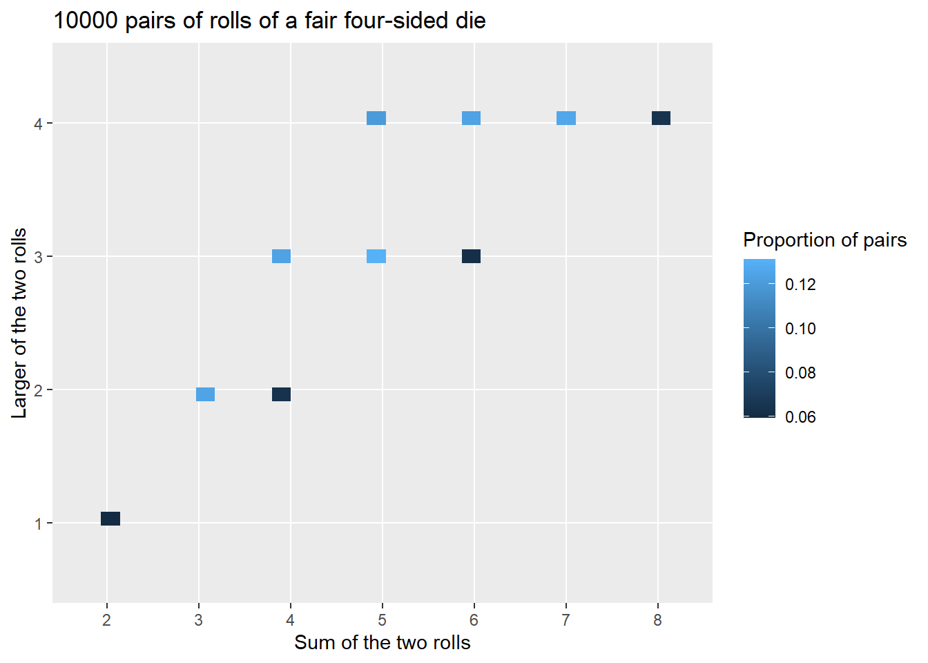
3.13 Case Study: Matching Problem

Dice rolling provides a simple scenario for us to introduce ideas, but it’s not very exciting. Now we’ll apply ideas from this chapter to investigate a more interesting problem: the matching problem. We’ll also see how we can combine Symbulate and Python code. Our analysis will illustrate sensitity analysis, where we see how probabilities, distributions, and expected values change as we vary parameters or assumptions.

Consider the matching problem for a general $n$: objects labeled $1, 2, 3, \ldots, n$ are placed at random in spots labeled $1, 2, 3, \ldots, n$ with spot 1 the correct spot for object 1, etc. Let the random variable $X$ count the number of objects (out of $n$) that are put back in the correct spot; $X$ is the number of “matches”. Let $\textrm{P}$ denote the probability measure corresponding to the assumption that the objects are equally likely to be placed in any spot, so that the $n!$ possible placements are equally.

We have previously considered the case $n=4$ (Example 2.2, Example 2.22, Exercise 2.15). By enumerating the $4! = 24$ possible outcomes (see Table 2.2 and Table 2.9) we found the distribution of $X$ when $n=4$, displayed in Table 3.17 and Figure 3.36. When $n=4$ the probability of at least one match is 0.625, and the expected value of $X$ is 1.

Table 3.17: Distribution of $X$, the number of matches in the matching problem with $n=4$ and uniformly random placement of objects in spots.

x	P(X=x)
0	0.3750
1	0.3333
2	0.2500
4	0.0417

Figure 3.36: Distribution of $X$, the number of matches in the matching problem with $n=4$ and uniformly random placement of objects in spots.

When $n=4$ we could enumerate the $4!=24$ possible outcomes, but such a strategy is not feasible for a general $n$. For example, if $n=60$ then there are $60! \approx 10^{82}$ possible outcomes, which is about the total number of atoms in the observable universe. Therefore we need other strategies to investigate the problem.

We’ll use simulation to perform a sensitivity analysis to investigate how the distribution of $X$, the probability of at least one match, and the expected value of $X$ depend on $n$.

Warning

This is not really a warning but before proceeding, stop to think: what do you expect? How do you expect the probability of at least one match to depend on $n$? Will the probability increase, decrease, or stay about the same as $n$ gets larger? What about the expected value of the number of matches? It’s always a good idea to think about a problem and make some initial guesses before just jumping into calculations or simulations.

Example 3.36 For the matching problem for a given $n$, describe in detail how you would use simulation to approximate:

The distribution of $X$
$\textrm{P}(X \ge 1)$
$\textrm{E}(X)$.

Solution (click to expand)

Solution 3.36. We could use a box model.

The box has $n$ tickets, labeled $1, 2, \ldots, n$, one for each object.
An outcome is simulated by selecting $n$ tickets from the box without replacement and recording their order, e.g., (2, 1, 3, 4) if $n=4$.
Let $x$ be the number of matches for the simulated outcome, e.g., $x=2$ for outcome (2, 1, 3, 4).
The above two steps consist of one repetition, yielding one realized value of the random variable $X$.
Repeat these steps many times to obtain many simulated values of $X$.

Summarize the simulated values of $X$ and their relative frequencies to approximate the distribution of $X$.
Count the number of repetitions on which $X\ge 1$ and divide by the total number of repetitions to approximate $\textrm{P}(X\ge 1)$, the probability of at least one match.
We have seen that an expected value can be interpreted as a long run average value. To approximate $\textrm{E}(X)$, compute the average of the many simulated $X$ values—sum all simulated $X$ values and divide by the number of simulated $X$ values.

We’ll start by coding a simulation for $n=4$ so we can compare our simulation results to the analytical results to check that our simulation process is working correctly. Since Python uses zero-based indexing, we label the objects $0, 1, \ldots, n-1$.

n = 4

labels = list(range(n)) # list of labels [0, ..., n-1]
labels

[0, 1, 2, 3]

Now we define the box model and simulate a few outcomes. Note that replace = False.

P = BoxModel(labels, size = n, replace = False)

P.sim(5)

Index	Result
0	(2, 3, 0, 1)
1	(2, 1, 0, 3)
2	(0, 3, 1, 2)
3	(3, 2, 1, 0)
4	(0, 3, 1, 2)

We simulate many outcomes to check that they are roughly equally likely.

P.sim(24000).tabulate()

Outcome	Frequency
(0, 1, 2, 3)	1000
(0, 1, 3, 2)	913
(0, 2, 1, 3)	987
(0, 2, 3, 1)	1036
(0, 3, 1, 2)	1036
(0, 3, 2, 1)	1013
(1, 0, 2, 3)	990
(1, 0, 3, 2)	989
(1, 2, 0, 3)	992
(1, 2, 3, 0)	985
(1, 3, 0, 2)	1040
(1, 3, 2, 0)	1003
(2, 0, 1, 3)	1013
(2, 0, 3, 1)	989
(2, 1, 0, 3)	979
(2, 1, 3, 0)	993
(2, 3, 0, 1)	1020
(2, 3, 1, 0)	1010
(3, 0, 1, 2)	973
...	...
(3, 2, 1, 0)	1060
Total	24000

Remember that a random variable $X$ is a function whose inputs are the sample space outcomes. In this example the function “counts matches”, so would like to define $X$ as X = RV(P, count_matches). Unfortunately, such a function isn’t built in like sum or max, but we can write a custom count_matches Python function. The count_matches function below starts a counter at 0 and then goes spot-by-spot through each spot in the outcome and increments the counter by 1 any time there is a match (along the lines of the discussion in Section 2.3.4). Don’t worry too much about the Python syntax yet. What’s important is that we have defined a function that we can use to define a random variable.

def count_matches(outcome):
    count = 0
    for i in range(0, n, 1):
        if outcome[i] == labels[i]:
            count += 1
    return count
  
outcome = (1, 0, 2, 3) # an example outcome, with 2 matches
count_matches(outcome) # the function evaluated for the example outcome

Now we can use the function count_matches to define a Symbulate RV just like we have used sum or max.

X = RV(P, count_matches)

X((1, 0, 2, 3)) # evaluate X for the sample outcome

Warning: Calling an RV as a function simply applies the function that defines the RV to the input, regardless of whether that input is a possible outcome in the underlying probability space.
2

We can simulate many values of $X$ and use the simulated values to approximate the distribution of $X$, the probability of at least one match, and the expected value of $X$.

x = X.sim(10000)

x.tabulate(normalize = True)

Value	Relative Frequency
0	0.3752
1	0.3374
2	0.2447
4	0.0427
Total	1.0

x.plot()
plt.show()

x.count_geq(1) / x.count()

0.6248

x.sum() / x.count()

0.9976

The simulated distribution of $X$ is close to the true distribution in Table 3.17 when $n=4$; the simulated relative frequencies are within the margin of error (about 0.01-0.02 for 10000 simulated values) of the true probabilities. We also see that the average of the simulated $X$ values is around the theoretical expected value of 1.

It appears that our simulation is working properly for $n=4$. To investigate a different value of $n$, we simply need to revise the line n = 4. Because we want to investigate many values of $n$, we wrap all the above code in a Python function matching_sim which takes n as an input⁴¹ and outputs our objects of interest: a plot of the distribution of simulated $X$ values, the approximation of $\textrm{P}(X \ge 1)$, and the approximation of $\textrm{E}(X)$.


def matching_sim(n):
  
    labels = list(range(n))
    
    def count_matches(omega):
        count = 0
        for i in range(0, n, 1):
            if omega[i] == labels[i]:
                count += 1
        return count
    
    P = BoxModel(labels, size = n, replace = False)
    X = RV(P, count_matches)
    
    x = X.sim(10000)
    
    plt.figure()
    x.plot('impulse')
    plt.show()
    
    return x.count_geq(1) / x.count(), x.sum() / x.count()

For example, for $n=4$ we simply call

matching_sim(4)

(0.6262, 1.0127)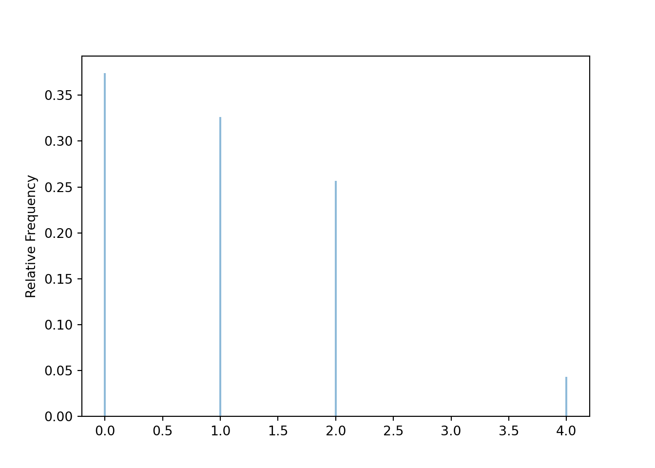

Now we can easily investigate different values of $n$. For example, for $n=10$ we see that the approximate probability of at least one match is around 0.63 and the approximate expected value of the number of matches is around 1.

matching_sim(10)

(0.6315, 0.9973)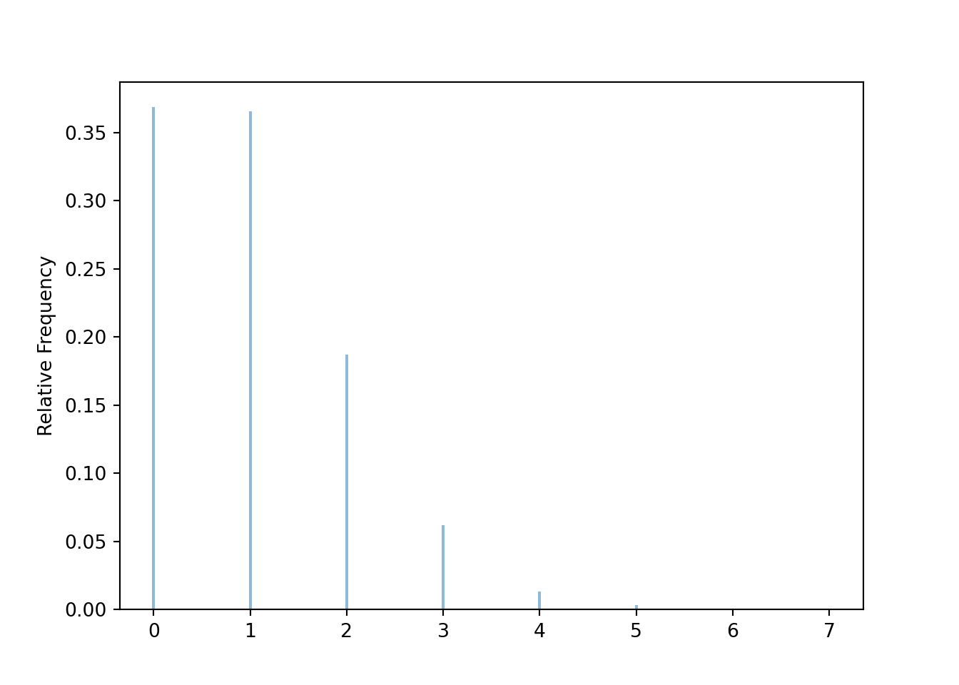

We can use a for loop to automate the process of changing the value of $n$, running the simulation, and recording the results. If ns is the list of $n$ values of interest we basically just need to run

for n in ns:
    matching_sim(n)

In Python we can also use list comprehension

[matching_sim(n) for n in ns]

The table below summarizes the simulation results for $n=4, \ldots, 10$. The first line defines the values of $n$, and the second line implements the for loop. We have used the Python package tabulate to add a little formatting to the table. (Don’t confuse this with the Symbulate tabulate method!) Note that we have temporarily redefined matching_sim to remove the lines that produced the plot, but we have not displayed the revised code here. (We will bring the plot back soon.)

from tabulate import tabulate

ns = list(range(4, 11, 1))

results = [matching_sim(n) for n in ns]

print(tabulate({'n': ns,
                'Approximate P(X >= 1), Approximate E(X)': results},
               headers = 'keys', floatfmt=".3f"))

  n  Approximate P(X >= 1), Approximate E(X)
---  -----------------------------------------
  4  (0.6118, 0.9617)
  5  (0.6288, 0.9966)
  6  (0.6347, 1.0059)
  7  (0.6434, 1.0333)
  8  (0.6323, 0.9958)
  9  (0.6291, 1.0003)
 10  (0.6281, 0.9985)

Stop and look at the table; what do you notice? How do the probability of at least one match and the expected value of the number of matches depend on $n$? They don’t! Well, maybe they do, but they don’t appear to change very much with $n$ after we take into account simulation margin of error⁴² of about 0.01-0.02. It appears that regardless of the value of $n$, the probability of at least one match is around 0.63 and the expected value of the number of matches is around 1.

If we’re interested in more values of $n$, we just repeat the same process with a longer list of ns. The code below uses the Python package Matplotlib to create a plot of the probability of at least one match and the expected value of the number of matches versus $n$. While there is some natural simulation variability, we see that the probability of at least one match (about 0.63) and the expected value of the number of matches (about 1) essentially do not depend on $n$!

from matplotlib import pyplot as plt

ns = list(range(4, 101, 1))

results = [matching_sim(n) for n in ns]

plt.figure()
plt.plot(ns, results)
plt.legend(['Approximate E(X)', 'Approximate P(X >= 1)'])
plt.xlabel('n')
plt.ylabel('value')
plt.show()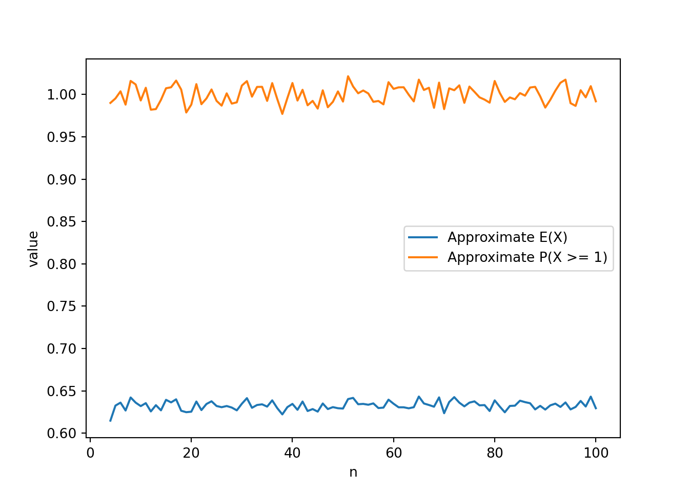

What about the distribution of $X$? This Colab notebook contains code for investigating how the distribution of $X$ depends on $n$. The basic simulation code is identical to what we have already seen. The notebook adds a few lines to create a Jupyter widget, which produces an interactive plot (with some additional formatting) of the distribution; you can change the slider to see how the distribution of $X$ changes with $n$. Take a few minutes to play with the slider; what do you see?

You should see that unless $n$ is really small (like 5 or less) the distribution of $X$ is basically the same for any value of $n$! We will see soon that the number of matches follows, approximately, a “Poisson(1)” distribution, regardless of the value of $n$ (unless $n$ is really small). In particular, the probability of 0 matches is approximately equal to 0.37, and also approximately equal to the probability of exactly 1 match.

Table 3.18: Approximate distribution of $X$, the number of matches in the matching problem for general $n$ and uniformly random placement of objects in spots.

x	P(X=x)
0	0.3679
1	0.3679
2	0.1839
3	0.0613
4	0.0153
5	0.0031
6	0.0005
7	0.0001

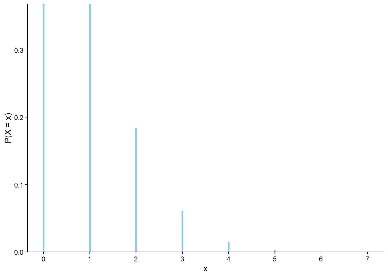
Figure 3.37: Approximate distribution of $X$, the number of matches in the matching problem for general $n$ and uniformly random placement of objects in spots.

Summarizing, our sensitivity analysis⁴³ of the matching problem reveals that, unless $n$ is really small,

the probability of at least one match does is approximately 0.632
the expected value—that is, long run average— of the number of matches is approximately 1
the distribution of the number of matches is approximately the “Poisson(1)” distribution.

We will investigate these observations further later. For now, marvel at the fact that no matter if there are 10 or 100 or 1000 people in you next Secret Santa gift exchange, it’s roughly 2 to 1 odds in favor of somebody drawing their own name!

3.13.1 Exercises

Exercise 3.28 Katniss throws a dart at a circular dartboard with radius 12 inches. Suppose that the dartboard is on a coordinate plane, with the center of the dartboard at (0, 0) and the north, south, east, and west edges, respectively, at coordinates (0, 12), (0,-12), (12, 0), (-12, 0). When the dart hits the board its $(X, Y)$ coordinates are recorded.

Assume that $X$ and $Y$ each follow a Normal(0, $\sigma$), independently. Note that it is possible for the dart to land off the board. Let $R$ be the distance (inches) from the location of the dart to the center of the dartboard.

Combine Symbulate and Python code to perform a sensivity analysis of how the following depend on $\sigma$ (for say values of $\sigma<5$):

$\textrm{P}(R < 1)$
$\textrm{P}(R > 12)$
$\textrm{E}(R)$

3.14 Simulating from distributions

The distribution of a random variable specifies the long run pattern of variation of values of the random variable over many repetitions of the underlying random phenomenon, or the relative degree of likelihood of possible values. The distribution of a random variable $X$ can be approximated by

simulating an outcome of the underlying random phenomenon $\omega$ according to the assumptions encoded in the probability measure $\textrm{P}$
observing the value of the random variable for that outcome $X(\omega)$
repeating this process many times
then computing relative frequencies involving the simulated values of the random variable to approximate probabilities of events involving the random variable, e.g., $\textrm{P}(X\le x)$.

We have carried out this process for several examples, including the dice rolling example in Section 3.1 and Section 3.3, where each repetition involved simulating a pair of rolls (outcome $\omega$) and then finding the sum ($X(\omega)$) and max ($Y(\omega)$).

Now we’ll discuss another method for simulating values of a random variable.

Example 3.37 Recall Example 2.41, Table 2.14, and Table 2.15.

Construct a spinner to represent the marginal distribution of $X$.
How could you use the spinner from the previous part to simulate a value of $X$?
Construct a spinner to represent the marginal distribution of $Y$.
How could you use the spinner from the previous part to simulate a value of $Y$?
Donny Don’t says: “Great! I can simulate an $(X, Y)$ pair just by spinning the spinner in Figure 3.38 (a) to generate $X$ and the one in Figure 3.38 (b) to generate $Y$.” Is Donny correct? If not, can you help him see why not?
Construct a single spinner for simulating $(X, Y)$ pairs with the proper joint distribution.

Solution (click to expand)

Solution 3.37.

The spinner in Figure 3.38 (a) represents the marginal distribution of $X$ in Table 2.14.
Just spin it! The spinner returns the possible values of $X$ according to the proper probabilities. If we’re interested in simulating the sum of two rolls of a fair four-sided dice, we don’t have to roll the dice; we can just spin the $X$ spinner once.
The spinner in Figure 3.38 (b) represents the marginal distribution of $Y$ in Table 2.15.
Just spin it! The spinner returns the possible values of $Y$ according to the proper probabilities. If we’re interested in simulating the larger of two rolls of a fair four-sided dice, we don’t have to roll the dice; we can just spin the $Y$ spinner once.
Donny is incorrect. Yes, spinning the $X$ spinner in Figure 3.38 (a) will generate values of $X$ according to the proper marginal distribution, and similarly with Figure 3.38 (b) and $Y$. However, spinning each of the spinners will not produce $(X, Y)$ pairs with the correct joint distribution. For example, Donny’s method could produce $X=2$ and $Y=4$, which is not a possible $(X, Y)$ pair. Donny’s method treats the values of $X$ and $Y$ as if they were independent; the result of the $X$ spin would not change what could happen with the $Y$ spin (since the spins are physically independent). However, the $X$ and $Y$ values are related. For example, if $X=2$ then $Y$ must be 1; if $X=4$ then $Y$ must be 2 or 3; etc.
See the spinner in Figure 3.38 (c) which would properly simulate $(X, Y)$ pairs according to the joint distribution.

(a) The marginal distribution of $X$; see Table 2.14

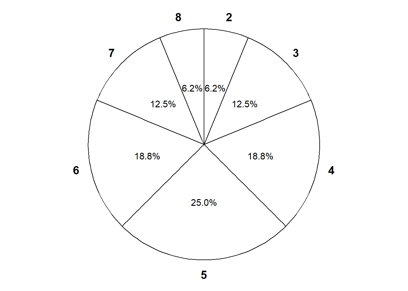
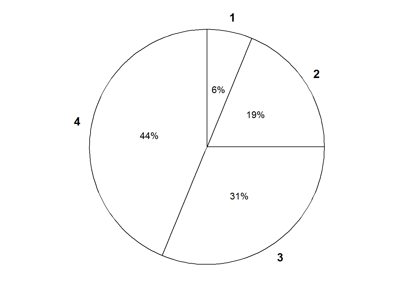
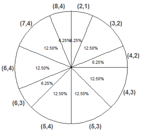
In principle, there are always two ways of simulating a value $x$ of a random variable $X$.

Simulate from the probability space. Simulate an outcome $\omega$ from the underlying probability space and set $x = X(\omega)$.
Simulate from the distribution. Simulate a value $x$ directly from the distribution of $X$.

The “simulate from the distribution” method corresponds to constructing a spinner representing the distribution of $X$ and spinning it once to generate $x$.

Example 3.38 Donny Don’t says: “The ‘simulate from the distribution’ method is dumb. In order to use it, I first need to know the distribution. But the whole point of simulation is to approximate a distribution. If I know the distribution, why do I need to approximate it?” How would you respond to Donny? Hint: it might help to consider the brown bag analogy in Section 2.3.2. It might also help to consider how we use simulation in the meeting problem in this chapter.

Solution (click to expand)

Solution 3.38. Yes, this method does require that the distribution of $X$ is known. However, in many situations we assume a distribution for a random variable directly, without specifying the underlying probability space. This is what we did in the meeting problem whenever we assumed a Uniform(0, 60) or Normal(30, 10) distribution for arrival times. Even Donny himself tried to implement the simulate from the distribution method in Example 3.31.

In many problems we often assume or identify distributions directly, without any mention of the underlying sample space or probability measure. Recall the brown bag analogy in Section 2.3.2. The probability space corresponds to the random selection of fruits to put in the bag. The random variable is weight. The distribution of weight can be obtained by randomly selecting fruits to put in the bag, weighing the bag, and then repeating this process many times to observe many weights. For example, maybe 10% of bags have weights less than 5 pounds, 75% of bags have weights less than 20 pounds, etc. We can observe the distribution of weights even if we don’t observe the actual fruits in the bag or fully specify the random phenomenon and its sample space.

Example 3.39 In Section 3.3 we saw the Symbulate code for the “simulate from the probability space” method in the dice rolling example. Now we consider the “simulate from the distribution method”.

Write the Symbulate code to define $X$ by specifying its marginal distribution.
Write the Symbulate code to define $Y$ by specifying its marginal distribution.
Can the code from the previous parts be combined to simulate $(X, Y)$ pairs?
Write the simulate code to define $(X, Y)$ by specifying the joint distribution.

Solution (click to expand)

Solution 3.39.

We simulate a value of $X$ from its marginal distribution by spinning the spinner in Figure 3.38 (a), which we can define via a BoxModel
Similarly, we simulate a value of $Y$ from its marginal distribution by spinning the spinner in Figure 3.38 (b), which we can define via a BoxModel
No. The previous parts only define the marginal distributions, and marginal distributions alone do not define the joint distribution.
We simulate an $(X, Y)$ pair from its joint distribution by spinning the spinner in Figure 3.38 (c), which we can define via a BoxModel whose tickets represent pairs.

We can define a BoxModel corresponding to each of the spinners in Figure 3.38, and then define a random variable with that distribution via RV(BoxModel(...)). Essentially, we define the random variable by specifying its distribution (spinner), rather than specifying the underlying probability space. Note that the default size argument in BoxModel is size = 1, so we have omitted it.

X = RV(BoxModel([2, 3, 4, 5, 6, 7, 8], probs = [1 / 16, 2 / 16, 3 / 16, 4 / 16, 3 / 16, 2 / 16, 1 / 16]))

x = X.sim(10000)

x.tabulate(normalize = True)

Value	Relative Frequency
2	0.0628
3	0.13
4	0.1813
5	0.2583
6	0.1877
7	0.1183
8	0.0616
Total	1.0

x.plot()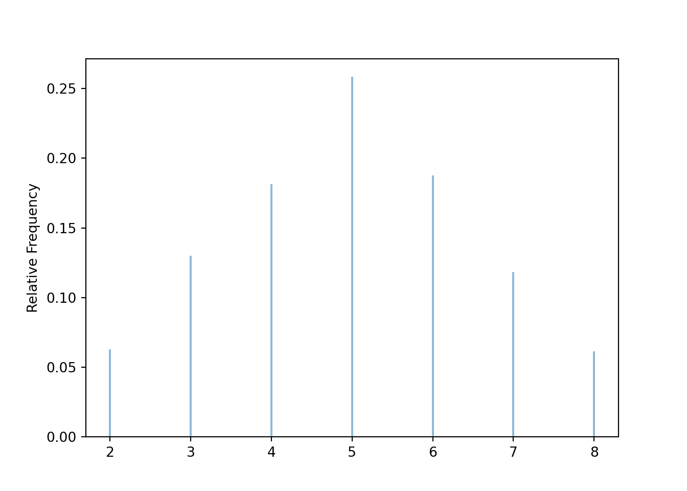

Similarly we can define $Y$ as

Y = RV(BoxModel([1, 2, 3, 4], probs = [1 / 16, 3 / 16, 5 / 16, 7 / 16]))

To simulate $(X, Y)$ pairs we need to specify the joint distribution.

xy_pairs = [(2, 1), (3, 2), (4, 2), (4, 3), (5, 3), (5, 4), (6, 3), (6, 4), (7, 4), (8, 4)]

pxy = [1/16, 2/16, 1/16, 2/16, 2/16, 2/16, 1/16, 2/16, 2/16, 1/16]

X, Y = RV(BoxModel(xy_pairs, probs = pxy, size = 1))

(X & Y).sim(10000).tabulate(normalize = True)

Value	Relative Frequency
(2, 1)	0.0628
(3, 2)	0.1247
(4, 2)	0.0616
(4, 3)	0.1219
(5, 3)	0.1182
(5, 4)	0.1288
(6, 3)	0.0647
(6, 4)	0.1267
(7, 4)	0.1262
(8, 4)	0.0644
Total	1.0

BoxModel with the probs option can be used to define general discrete distributions (when there are finitely many possible values). Many commonly encountered distributions have special names, and in Symbulate we can define a random variable to have a specific named distribution through code of the form RV(Distribution(parameters)); for example X = RV(Uniform(0, 60)) or X = RV(Normal(30, 10)). Think of code like X = RV(Normal(30, 10)) as “$X$ is a random variable with a Normal(30, 10) distributon”.

3.15 Do not confuse a random variable with its distribution

We close this chapter with a warning.

Warning

Do not confuse a random variable with its distribution.

A random variable measures a numerical quantity which depends on the outcome of a random phenomenon. The distribution of a random variable specifies the long run pattern of variation of values of the random variable over many repetitions of the underlying random phenomenon⁴⁴. The distribution of a random variable can be approximated by simulating an outcome of the random process, observing the value of the random variable for that outcome, repeating this process many times, and summarizing the results. But a random variable is not its distribution.

Recall the brown bag analogy in Section 2.3.2. The probability space corresponds to the random selection of fruits to put in the bag. The random variable is weight. The distribution of weight can be obtained by randomly selecting fruits to put in the bag, weighing the bag, and then repeating this process many times to observe many weights, summarize the values, and describe the pattern of variability (e.g., 10% of bags have weights less than 5 pounds, 75% of bags have weights less than 20 pounds, etc). But the random variable is like the scale itself.

A distribution is determined by:

The underlying probability measure $\textrm{P}$, which represents all the assumptions about the random phenomenon.
The random variable $X$ itself, that is, the function which maps sample space outcomes to numbers.

Changing either the probability measure or the random variable itself can change the distribution of the random variable. For example, consider the sample space of two rolls of a fair four-sided die. In each of the following scenarios, the random variable $X$ has a different distribution.

The die is fair and $X$ is the sum of the two rolls
The die is fair and $X$ is the larger of the two rolls
The die is weighted to land on 1 with probability 0.1 and 4 with probability 0.4 and $X$ is the sum of the two rolls.

In particular,

$X$ takes the value 2 with probability $1/16$
$X$ takes the value 2 with probability $3/16$
$X$ takes the value 2 with probability 0.01.

In (1) and (2), the probability measure is the same (fair die) but the function defining the random variable is different (sum versus max). In (1) and (3), the function defining the random variable is the same, and the sample space of outcomes is the same, but the probability measure is different.

We often specify the distribution of a random variable directly without explicit mention of the underlying probability space or function defining the random variable. For example, in the meeting problem we might assume that arrival times follow a Uniform(0, 60) or a Normal(30, 10) distribution. In situations like this, you can think of the probability space as being the distribution of the random variable and the function defining the random variable to be the identity function. In other words, we construct a spinner to represent the distribution of the random variable and spin it to simulate a value of the random variable.

Example 3.40 Donny Dont is thoroughly confused about the distinction between a random variable and its distribution. Help him understand by by providing a simple concrete example of two different random variables $X$ and $Y$ that have the same distribution. Can you think of $X$ and $Y$ for which $\textrm{P}(X = Y) = 0$? How about a discrete example and a continuous example?

Solution (click to expand)

Solution 3.40. Roll two fair four-sided dice and let $U_1$ be the result of the first roll and $U_2$ the result of the second roll. Then $U_1$ and $U_2$ have the same distribution; each takes values 1, 2, 3, 4 with equal probability. However, these are two different random variables; one measure the first roll and one measure the second. If the first roll is 4 and the second roll is 3, then $U_1=4$ and $U_2=3$, which are not the same.

Another discrete example: Flip a fair coin 3 times and let $X$ be the number of heads and $Y$ be the number of tails. Then $X$ and $Y$ have the same distribution, because the coin is fair, roughly heads and tails would have the same long run pattern of variability. (In this case each of $X$ and $Y$ takes values 0, 1, 2, 3 with probability 1/8, 3/8, 3/8, 1/8.) But $X$ and $Y$ are not the same random variable; they are measuring different things. If the outcome is HHT then $X$ is 2 but $Y$ is 1. In this case $\textrm{P}(X = Y)=0$; in an odd number of flips it’s not possible to have the same number of heads and tails on any single outcome.

A continuous example follows.

In some cases of the meeting time problem we assumed the distribution of Regina’s arrival time $R$ is Uniform(0, 60) and the distribution of Cady’s arrival time $Y$ is Uniform(0, 60), in which case $R$ and $Y$ have the same distribution. But these are two random variables; one measures Regina’s arrival time and one measure Cady’s. If Regina and Cady met every day for a year, then the day-to-day pattern of Regina’s arrival times would look like the day-to-day pattern of Cady’s arrival times. But on any given day, their arrival times would not be the same, since $R$ and $Y$ are continuous random variables so $\textrm{P}(R = Y) = 0$.

A distribution, like a spinner, is a blueprint for simulating values of the random variable. If two random variables have the same distribution, you could use the same spinner to simulate values of either random variable. But a distribution is not the random variable itself.

Two random variables can have the same (long run) distribution, even if the values of the two random variables are never equal on any particular repetition (outcome). If $X$ and $Y$ have the same distribution, then the spinner used to simulate $X$ values can also be used to simulate $Y$ values; in the long run the patterns would be the same.

At the other extreme, two random variables $X$ and $Y$ are the same random variable only if for every outcome of the random phenomenon the resulting values of $X$ and $Y$ are the same. That is, $X$ and $Y$ are the same random variable only if they are the same function: $X(\omega)=Y(\omega)$ for all $\omega\in\Omega$. It is possible to have two random variables for which $\textrm{P}(X=Y)$ is large, but $X$ and $Y$ have different distributions.

Example 3.41 Explain why each of the following random variables has the same distribution.

$X$ is the number of Tails in three flips of a fair coin
$Y$ is the number of Tails in three flips of a fair coin
$Z$ is the number of even numbers rolled in three rolls of a fair six-sided die
$W$ is the number of females in three human births, selected randomly and independently, assuming males and females are equally likely⁴⁵

Solution (click to expand)

Solution 3.41. Each of these situations involves a different sample space of outcomes (coins, dice, births) with a random variable which counts different things (Heads, Tails, evens, boys). But all the scenarios have some general features in common:

There are 3 “trials” (3 flips, 3 rolls, 3 babies)
Each trial can be classified as “success”⁴⁶ (Tails, even, female) or not.
Each trial is equally likely to result in success or not (fair coin, fair die, assuming boys and girls are equally likely)
The trials are independent. For coins and dice the trials are physically independent. For births independence follows from random selection from a large population.
The random variable counts the number of successes in the 3 trials (number of H, number of T, number of even rolls, number of female babies).

Each situation can be simulated by putting 2 tickets in a box labeled success or not, drawing 3 tickets with replacement, counting the number of successes drawn, and repeating many times. All of these scenarios are probabilitistically the same, so each random variable would have the same long run pattern of variability.

Many commonly encountered distributions have special names. For example, the common distribution in Example 3.41 is called the “Binomial(3, 0.5)” distribution. If a random variable has a Binomial(3, 0.5) distribution then it takes the possible values 0, 1, 2, 3, with respective probability 1/8, 3/8, 3/8, 1/8. (We will study Binomial distributions in more detail later.)

Example 3.41 illustrates that knowledge that a random variable has a specific distribution (e.g., Binomial(3, 0.5)) does not necessarily convey any information about the underlying outcomes or random variable (function) being measured.

The scenarios involving $W, X, Y, Z$ in Example 3.41 illustrate that two random variables do not have to be defined on the same sample space in order to determine if they have the same distribution. This is in contrast to computing quantities like $\textrm{P}(X=Y)$: $\{X=Y\}$ is an event which cannot be investigated unless $X$ and $Y$ are defined for the same outcomes. For example, you could not estimate the probability that a student has the same score on both SAT Math and Reading exams unless you measured pairs of scores for each student in a sample. However, you could collect SAT Math scores for one set of students to estimate the marginal distribution of Math scores, and collect Reading scores for a separate set of students to estimate the marginal distribution of Reading scores, and see if those two marginal distributions are the same.

Example 3.42 Suppose that $X$, $Y$, and $Z$ all have the same distribution. Donny Dont says

The pair $(X, Y)$ has the same joint distribution as the pair $(X, Z)$.
$X+Y$ has the same distribution as $X+Z$.
$X+Y$ has the same distribution as $X+X=2X$.

Determine if each of Donny’s statements is correct. If not, explain why not using a simple example (say a coin flipping situation).

Solution (click to expand)

Solution 3.42. First of all, Donny’s statements wouldn’t even make sense unless the random variables were all defined on the same probability space. For example, if $X$ is SAT Math score and $Y$ is SAT reading score it doesn’t makes sense to consider $X+Y$ unless $(X, Y)$ pairs are measured for the same students. But even assuming the random variables are defined on the same probability space, we can find counterexamples to Donny’s statements.

As just one example, flip a fair coin 4 times and let

$X$ be the number of heads in flips 1 through 3
$Y$ be the number of tails in flips 1 through 3
$Z$ be the number of heads in flips 2 through 4.

The joint distribution of $(X, Y)$ is not the same as the joint distribution of $(X, Z)$. For example, $(X, Y)$ takes the pair $(3, 3)$ with probability 0, but $(X, Z)$ takes the pair $(3, 3)$ with nonzero probability (1/16).
The distribution of $X+Y$ is not the same as the distribution of $X+Z$; $X+Y$ is 3 with probability 1, but the probability that $X+Z$ is 3 is less than 1 (4/16).
The distribution of $X+Y$ is not the same as the distribution of $2X$; $X+Y$ is 3 with probability 1, but $2X$ takes values 0, 2, 4, 6 with nonzero probability.

Remember that a joint distribution is a probability distribution on pairs of values. Just because $X_1$ and $X_2$ have the same marginal distribution, and $Y_1$ and $Y_2$ have the same marginal distribution, doesn’t necessary imply that $(X_1, Y_1)$ and $(X_2, Y_2)$ have the same joint distributions. In general, information about the marginal distributions alone is not enough to determine information about the joint distribution. Comparing Example 2.41 and Example 2.43 provides another example of two scenarios with the same marginal distributions but different joint distributions.

The distribution of any random variable obtained via a transformation of multiple random variables will depend on the joint distribution of the random variables involved; for example, the distribution of $X+Y$ depends on the joint distribution of $X$ and $Y$.

Example 3.43 Spin the Uniform(0, 1) spinner (see Figure 2.1) twice and let $U_1$ be the result of the first spin and $U_2$ the result of the second. For each of the following pairs of random variables, determine whether or not they have the same distribution as each other. No calculations necessary; just think conceptually.

$U_1$ and $U_2$
$U_1$ and $1-U_1$
$U_1$ and $1+U_1$
$U_1$ and $U_1^2$
$U_1+U_2$ and $2U_1$
$U_1$ and $1-U_2$
Is the joint distribution of $(U_1, 1-U_1)$ the same as the joint distribution of $(U_1, 1 - U_2)$?

Solution (click to expand)

Solution 3.43.

Yes, each has a Uniform(0, 1) distribution.
Yes, each has a Uniform(0, 1) distribution. For $u\in[0, 1]$, $1-u\in[0, 1]$, so $U_1$ and $1-U_1$ have the same possible values, and a linear rescaling does not change the shape of the distribution. Changing from $U_1$ to $1-U_1$ essentially amounts to switching the [0, 1] labels on the spinner from clockwise to counterclockwise.
No, the two variables do not have the same possible values. The shapes would be similar though; $1+U_1$ has a Uniform(1, 2) distribution.
No, a non-linear rescaling generally changes the shape of the distribution. For example, $\textrm{P}(U_1\le0.49) = 0.49$, but $\textrm{P}(U_1^2 \le 0.49) = \textrm{P}(U_1 \le 0.7) = 0.7$ Squaring a number in [0, 1] makes the number even smaller, so the distribution of $U_1^2$ places higher density on smaller values than $U_1$ does.
No, $U_1+U_2$ has a triangular shaped distribution on (0, 2) with a peak at 1. (The shape is similar to that of the distribution of $X$ in ?sec-sim-transform-joint), but the possible values are (0, 2) rather than (2, 8).) But $2U_1$ has a Uniform(0, 2) distribution. Do not confuse a random variable with its distribution. Just because $U_1$ and $U_2$ have the same distribution, you cannot replace $U_2$ with $U_1$ in transformations. The random variable $U_1+U_2$ is not the same random variable as $2U_1$; spinning a spinner and adding the spins will not necessarily produce the same value as spinner a spinner once and multiplying the value by 2.
Yes, just like $U_1$ and $1-U_2$ have the same distribution.
No. The marginal distributions are the same, but the joint distribution of $(U_1, 1-U_1)$ places all density along a line, while the joint density of $(U_1, 1-U_2)$ is distributed over the whole two-dimensional region $[0, 1]\times[0,1]$.

Do not confuse a random variable with its distribution. This is probably getting repetitive by now, but we’re emphasizing this point for a reason. Many common mistakes in probability problems involve confusing a random variable with its distribution. For example, we will soon that if a continuous random variable $X$ has probability density function $f(x)$, then the probability density function of $X^2$ is NOT $f(x^2)$ nor $(f(x))^2$. Mistakes like these, which are very common, essentially involve confusing a random variable with its distribution. Understanding the fundamental difference between a random variable and its distribution will help you avoid many common mistakes, especially in problems involving a lot of calculus or mathematical symbols.

3.16 Chapter exercises

TBA

In most situations we’ll encounter in this book, the “set up” step requires the most work and the most computer programming, while the “simulate” and “summarize” steps are usually straightforward. In many other cases, these steps can be challenging. Complex set ups often require sophisticated methods, such MCMC (Markov Chain Monte Carlo) algorithms, to efficiently simulate realizations. Effectively summarizing high dimensional simulation output often requires the use of multivariate statistics and visualizations.↩︎
Our use of “box models” is inspired by (Freedman, Pisani, and Purves 2007).↩︎
“With replacement” always implies replacement at a uniformly random point in the box. Think of “with replacement” as “with replacement and reshuffling” before the next draw.↩︎
If we’re repeating something many times, do we perform “a simulation” or “many simulations”? Throughout, “a simulation” refers to the collection of results corresponding to repeatedly artificially recreating the random process. “A repetition” refers to a single artificial recreation resulting in a single simulated outcome. We perform a simulation which consists of many repetitions.↩︎
Technically, a Normal(30, 10) distribution allows for values outside the [0, 60] interval, but the probability is small, roughly 0.003.↩︎
We primarily view a Symbulate probability space as a description of the probability model rather than an explicit specification of the sample space $\Omega$. For example, we define a BoxModel instead of creating a set with all possible outcomes. We tend to represent a probability space with P, even though this is a slight abuse of notation (since $\textrm{P}$ typically refers to a probability measure).↩︎
The default argument for replace is True, so we could have just written BoxModel([1, 2, 3, 4], size = 2).↩︎
There is an additional argument order_matters which defaults to True, but we could set it to False for unordered pairs.↩︎
We generally use names in our code that mirror and reinforce standard probability notation, e.g., uppercase letters near the end of the alphabet for random variables, with corresponding lowercase letters for their realized values. Of course, these naming conventions are not necessary and you are welcome to use more descriptive names in your code. For example, we could have named the probability space DiceRolls and the random variables DiceSum and DiceMax rather than P, X, Y. Whatever you do, we encourage you to use names that distinguish the objects themselves from their simulated values, e.g. Dice_Sum for the random variable and dice_sum_sim for the simulated values.↩︎
Technically & joins two RVs together to form a random vector. While we often interpret Symbulate RV as “random variable”, it really functions as “random vector”.↩︎
You might try (P & X).sim(10). But P is a probability space object, and X is an RV object, and & can only be used to join like objects together. Much like in probability theory in general, in Symbulate the probability space plays a background role, and it is usually random variables we are interested in.↩︎
The components of an RV can also be accessed using brackets. U1, U2 = RV(P) is shorthand for
U = RV(P); U1 = U[0]; U2 = U[1].↩︎
We could have actually defined Z = (X - 5) ** 2 here. We’ll see examples where the apply syntax is necessary later.↩︎
We can also define U = RV(P) and then X = U.apply(sum).↩︎
We can also define U = RV(P) and then X = U.apply(max).↩︎
Braces {} are used here because this defines a Python dictionary. But don’t confuse this code with set notation.↩︎
Careful: don’t confuse Uniform(a, b) with DiscreteUniform(a, b). Uniform(a, b) corresponds to the continuous interval $[a, b]$.↩︎
We would typically only include the values observed in the simulation in the summary. However, we include 4 and 8 here because if we had performed more repetitions we would have observed these values.↩︎
“Normalize” is used in the sense of Section 1.3 and refers to rescaling the values so that they add up to 1 but the ratios are preserved.↩︎
For discrete random variables 'impulse' is the default plot type. Like .tabulate(), the .plot() method also has a normalize argument; the default is normalize=True.↩︎
In 10000 flips, the probability of heads on between 49% and 51% of flips is 0.956, so 98 out of 100 provides a rough estimate of this probability. We will see how to compute such a probability later.↩︎
This is difficult to see in Figure 3.12 due to the binning. But we can at least tell from Figure 3.12 that at most a handful of the 100 sets resulted in a proportion of heads exactly equal to 0.5.↩︎
Technically, we should say “a margin of error for 95% confidence of 0.01”. We’ll discuss “confidence” in a little more detail soon.↩︎
In 1,000,000 flips, the probability of heads on between 49.9% and 50.1% of flips is 0.955, and 91 out of 100 sets provides a rough estimate of this probability.↩︎
In 100 million flips, the probability of heads on between 49.99% and 50.01% of flips is 0.977, and 96 out of 100 sets provides a rough estimate of this probability.↩︎
One difference between RV and apply: apply preserves the type of the input object. That is, if apply is applied to a ProbabilitySpace then the output will be a ProbabilitySpace; if apply is applied to an RV then the output will be an RV. In contrast, RV always creates an RV.↩︎
Unfortunately, for techincal reasons, RV(P, count_eq(6) / N) will not work. It is possible to divide by N within RV if we define a custom function def rel_freq_six(x): return x.count_eq(6) / N and then define RV(P, rel_freq_six).↩︎
We will see the rationale behind this formula later. The factor 2 comes from the fact that for a Normal distribution, about 95% of values are within 2 standard deviations of the mean. Technically, the factor 2 corresponds to 95% confidence only when a single probability is estimated. If multiple probabilities are estimated simultaneously, then alternative methods should be used, e.g., increasing the factor 2 using a Bonferroni correction. For example, a multiple of 4 rather than 2 produces very conservative error bounds for 95% confidence even when many probabilities are being estimated.↩︎
In all the situations in this book the repetitions will be simulated independently. However, there are many simulation methods where this is not true, most notably MCMC (Markov Chain Monte Carlo) methods. The margin of error needs to be adjusted to reflect any dependence between simulated values.↩︎
See the footnotes in Section 1.2.1.↩︎
It can be shown that the standard deviation is always at least as big as the average absolute deviation. For a Normal distribution, the average absolute deviation is about 0.8 times the standard deviation.↩︎
If you have some familiarity with statistics, you might have seen a formula for variance or standard deviation that includes dividing by one less than the number values ($n-1$). Dividing by $n$ or $n-1$ could make a difference in a small sample of data. However, we will always be interested in long run averages, and it typically won’t make any practical difference whether we divide by say 10000 or 9999. We’ll always compute averages by dividing by the number of values that we’re summing.↩︎
Think Pythagorean theorem: it’s $a^2+b^2=c^2$. On the other hand, for absolute values we only have the triangle inequality $|a+b| \le |a| + |b|$.↩︎
We usually represent joint distributions as two-way tables, but for this problem it helps to think of a table with one row for each pair.↩︎
All of our simulations are based on independently simulated repetitions. More sophisticated methods, such as Markov chain Monte Carlo (MCMC) methods, allow dependent repetitions and can approximate conditional probabilities much more efficiently.↩︎
Age_Snapchat is a pair so Age_Snapchat[0] is the first component (Age) and Age_Snapchat[1] is the second component (Snapchat user).↩︎
In Symbulate, events being conditioned on need to be based on RVs. But the code shows that Symbulate has a pretty broad interpretation of what can be an RV.↩︎
.draw() is like .sim(1) but they have different properties. We will usually work with .sim() to actually run a simulation. .draw() is useful in situations like this where we have to build a custom probability space from scratch.↩︎
Python automatically treats True as 1 and False as 0, so the code (y < 3) effectively returns both True/False realizations of the event itself and 1/0 realizations of the corresponding indicator random variable.↩︎
We wrote this code to compare to the previous block that returned an error. Even though the revised code works, it’s clunky because we unpack the rolls and then rejoin them in random variable world and then unpack them again in simulation world. We could simplify a little by not unpacking and rejoining in random variable variable world, using U = RV(P); u1_and_u2 = U.sim(10). This still isn’t the preferred way to sum the rolls, but we’re just illustrating a few ways to work in both random variable world and simulation world.↩︎
Because of the way we defined count_matches we need to redefine it if we change n and labels, which is why count_matches is defined inside matching_sim.↩︎
The simulation margin of error for relative frequency of at least one match is about 0.01 based on 10000 simulated values. We haven’t discussed simulation margins of error when aproximating expected values yet. In this case, the margin of error for a single average based on 10000 simulated values is about 0.02.↩︎
We might also be interested in other sensitivity analyses, such as what if the objects are not placed uniformly at random in the spots.↩︎
A distribution can also be interpreted as a subjective assessment of relative likelihood or plausibility, but here we’ll focus on the long run relative frequency interpretation.↩︎
Which isn’t quite true.↩︎
There is no value judgment; sSuccess” just refers to whatever we’re counting. Did the thing we’re counting happen on this trial (“success) or not (”failure”). Success isn’t necessarily good.↩︎