7  Mathematics of Probability

We have already encountered many important concepts in probability. In this chapter, we’ll explore further the mathematics of probability.

7.1 Equally likely outcomes

In this section we’ll look more closely at how to compute probabilities when the outcomes in the sample space are equally likely. But a warning before proceeding: in most situations sample space outcomes are not equally likely! And even in case where the outcomes are equally, values of corresponding random variables are usually not. So beware that the results for probabilities in this section only apply in a limited number of special cases. However, some of the rules for counting outcomes will be useful even when outcomes are not equally likely.

For a sample space \(\Omega\) with finitely many possible outcomes, assuming equally likely outcomes corresponds to a probability measure \(\textrm{P}\) which satisfies

\[ \textrm{P}(A) = \frac{|A|}{|\Omega|} = \frac{\text{number of outcomes in $A$}}{\text{number of outcomes in $\Omega$}} \qquad{\text{when outcomes are equally likely}} \]

Example 7.1 Flip a coin 4 times and record the results in sequence. For example, HTHH indicates T on the second flip and H on the others. Let \(X\) be the number of H in the four flips. Assume that the coin is fair and the flips are independent.

1. Find the probability of the outcome HTHH.
2. Find the probability of the outcome HHHH.
3. Make a table of all the possible outcomes; there should be 16. Is it reasonable to assume the outcomes are equally likely? Explain.
4. Identify the possible values of \(X\). Are the values of \(X\) equally likely?
5. Compute and interpret \(\textrm{P}(X = 4)\).
6. Compute and interpret \(\textrm{P}(X=3)\).
7. Find the distribution of \(X\).
8. Suppose the coin were biased in favor of landing on H. Would the sample space change? Would the definition of \(X\) and its possible values change? Would the 16 outcomes be equally likely? Would the distribution of \(X\) change?

Solution (click to expand)

Solution 7.1.

1. Since the coin is fair, the probability of H on any single flip is 0.5, same as the probability of T. Since the flips are independent, we can find the probability of the sequence by multiplying the probability of H/T for each flip. The probability of HTHH is (0.5)(0.5)(0.5)(0.5) = 0.0625 = 1/16.
2. Similar to the previous part, the probability of H is 1/16.
3. See Table 7.1. Assuming that the flips are independent and the coin is fair is equivalent to assuming that the probability of any single outcome is 1/16. So yes, it is reasonable to assume equally likely outcomes given these assumptions.
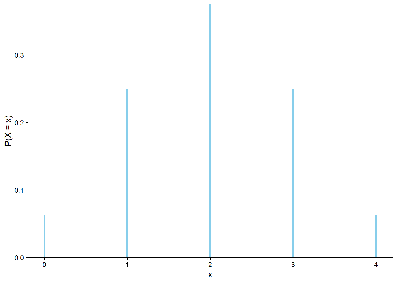
4. \(X\) can take values 0, 1, 2, 3, 4. (Don’t forget 0.) Even though the 16 possible sequences are equally likely, the values of \(X\) are not. For example, there are more outcomes that result in \(X=3\) than \(X=4\).
5. \(\textrm{P}(X = 4) = 1/16\) since there are 4 H in 4 flips if and only every flip is H, \(\{X = 4\} = \{HHHH\}\). Over many sets of 4 fair coin flips, about 6.25% of sets will result in 4 H. If you flip a coin 4 times, it is 15 times more likely to obtain fewer than 4 H than to obtain 4 H.
6. \(\textrm{P}(X = 3) = 4/16\) since there are 4 outcomes (out of 16 equally likely outcomes) with 3 H in 4 flips, \(\{X = 3\} = \{HHHT, HHTH, HTHH, THHH\}\). Over many sets of 4 fair coin flips, about 25% of sets will result in exactly 3 H. If you flip a coin 4 times, it is 3 times more likely to obtain something other than 3 H than to obtain 3 H.
7. The distribution can be represented in a table with the possible values \(x\) of \(X\), and \(\textrm{P}(X = x)\) for each possible \(x\). Since outcomes are equally, \(\textrm{P}(X = x)\) is the number of outcomes that satisfy the event \(\{X=x\}\) divided by 16, the total number of possible outcomes. See Table 7.2 and Figure 7.1.
8. If the coin were biased in favor of landing on H, the sample space wouldn’t change; there would still be 16 possible flip sequences. The definition of \(X\) and its possible values also would not change. However, the 16 outcomes would no longer be equally likely. For example, the probability of HHHH would be greater than that of TTTT The distribution of \(X\) would also change; for example, \(\textrm{P}(X = 4)\) would be greater than 1/16 and \(\textrm{P}(X = 0)\) would be less than 1/16.

Table 7.1: Table representing the outcomes of 4 flips of a coin, and \(X\), the number of H.

Outcome	X
HHHH	4
HHHT	3
HHTH	3
HTHH	3
THHH	3
HHTT	2
HTHT	2
HTTH	2
THHT	2
THTH	2
TTHH	2
HTTT	1
THTT	1
TTHT	1
TTTH	1
TTTT	0

Table 7.2: The marginal distribution of \(X\), the number of H in 4 flips of a fair coin.

x	P(X=x)
0	0.0625
1	0.2500
2	0.3750
3	0.2500
4	0.0625

Figure 7.1: The marginal distribution of \(X\), the number of H in 4 flips of a fair coin.

Remember that events often involve random variables. Even if the sample space outcomes are equally likely, the possible values of related random variables are usually not.

7.1.1 Some counting rules

Computing probabilities in the equally likely case reduces to just counting outcomes. In previous sections we often counted outcomes by enumerating them in a list. Of course, listing all the outcomes is unfeasible unless the sample space is very small. In this section we will see some formulas for counting in a few common situations.

All of the counting rules we’ll see are based on the multiplication principle for counting in Lemma 2.1. Review @#sec-language-counting-outcomes before proceeding.

Example 7.2 Suppose the board of directors of a corporation has identified 5 candidates — Ariana, Beyonce, Cardi, Drake, Elvis — for three executive positions: chief executive officer (CEO), chief financial officer (CFO), and chief operating officer (COO). In the interest of fairness, the board assigns 3 of the 5 candidates to the positions completely at random. No individual can hold more than one of the positions.

When calculating probabilities below, consider the sample space of all possible executive teams.

1. How many executive teams are possible?
2. What is the probability that Ariana is CEO, Beyonce is CFO, and Cardi is COO?
   
3. What is the probability that Ariana is CEO, Cardi is CFO, and Beyonce is COO?
   
4. What is the probability that Ariana is CEO and Beyonce is CFO?
5. What is the probability that Ariana is CEO?
6. What is the probability that Ariana is one of the executives?

Solution (click to expand)

Solution 7.2.

1. There are 5 choices for CEO, then 4 choices for CFO, then 3 choices for COO. So there are \(5\times 4 \times 3 = 60\) possible teams. The sample space consists of 60 possible outcomes. The order in which we make the choices doesn’t matter. We could have picked the CFO first then COO then CEO, still resulting in \(5\times 4\times3\) possible outcomes. What is important is that there are 3 distinct stages. Choosing Ariana as CEO is not the same as choosing Ariana as CFO.
2. If the selections are made uniformly at random, each of the 60 possible teams is equally likely. So the probability of any particular team, like this one, is 1/60.
3. The probability of any particular team is 1/60. But note that Ariana as CEO, Beyonce as CFO, and Cardi as COO is a different outcome than Ariana as CEO, Cardi as CFO, and Beyonce as COO
4. To construct a team with Ariana as CEO and Beyonce as CFO, there is one possible choice for CEO (Ariana), one possible choice for CFO (Beyonce) and three possible choices for COO, resulting in \(1\times 1\times 3\) teams that have Ariana as CEO and Beyonce as CFO. Since the outcomes are equally likely, the probability is 3/60.
5. To construct a team with Ariana as CEO, there is one possible choice for CEO (Ariana), four possible choicea for CFO, and three possible choices for COO, resulting in \(1\times 4\times 3=12\) teams that have Ariana as CEO. Since the outcomes are equally likely, the probability is 12/60=1/5. This makes sense because any of the five people is equally likely to be CEO.
6. The probability that Ariana is CEO is 12/60, similarly for CFO and COO. Since Ariana can’t hold more than one position, these events are disjoint, so the probability that Ariana is CEO or CFO or COO is \(3(12/60) = 3/5\).

Table 7.3: Ten of the 60 possible executive teams in Example 7.2

CEO	CFO	COO
A	B	C
A	C	B
B	A	C
B	C	A
C	A	B
C	B	A
A	B	D
A	B	E
A	C	D
A	C	E

In the previous example, the “stage” at which the person was chosen was important: there was a CEO stage, a CFO stage, and a COO stage. Choosing Ariana at the CEO stage, Beyonce at the CFO stage, and Cardi at the COO stage was a different outcome than choosing Ariana at the CEO stage, Cardi at the CFO stage, and Beyonce at the COO stage. When what happens at each stage matters, an outcome is often called an “ordered” arrangement. Again, “order” is perhaps a misnomer; it’s not that there’s a “first” and “second” and “third” stage, but rather that there are three distinct stages — CEO, CFO, COO.

The multiplication principle applies directly to situations which involve “ordered” or stage-wise counting, like the executive example. We employed the multiplication principle to find that there are \(5\times 4\times 3=60\) possible executive teams. The following formula generalizes this result.

Number of ordered arrangements. The number of ordered arrangements of \(k\) items, selected without replacement from a set of \(n\) distinct items is \[ n(n-1)(n-2)\cdots(n-k+1) = \frac{n!}{(n-k)!} \]

Recall the factorial notation: \(m!=m(m-1)(m-2)\cdots (3)(2)(1)\). For example, \(5!=5\times4\times3\times2\times1=120\). By definition, 0!=1.

Example 7.3 Your boss is forming a committee of 3 people for a new project team, and 5 people — Ariana, Beyonce, Cardi, Drake, Elvis— have volunteered to be on the committee. In the interest of fairness, 3 of the 5 people will be selected uniformly at random to form the committee.

1. How is this situation different from the executive team example?
2. How many possible committees consist of Ariana, Beyonce, Cardi? How many executive teams consisted of Ariana, Beyonce, Cardi?
3. How many different possible committees of 3 people can be formed from the 5 volunteers?

Solution (click to expand)

Solution 7.3.

1. There were distinct stages in the executive team example; selecting Ariana as CEO, Beyonce as CFO, and Cardi as COO was counted as a different outcome than selecting Ariana as CEO, Cardi as CFO, and Beyonce as COO. But when forming the committee we only need to know which three people were selected, not which stage or “order” they were selected in.
2. There is only one committee that consists of Ariana, Beyonce, Cardi. But there were 6 executive teams that consisted of Ariana, Beyonce, Cardi. See Table 7.4. To have a team with these three people, there are 3 choices for who is CEO, then 2 choices for COO, then 1 choice for COO, for a total of \(3\times2\times1=6\) possible teams consisting of Ariana, Beyonce, Cardi.
3. There were 60 possible “ordered” outcomes, but counting in an “ordered” way overcounts the number of committees by a factor of 6. Counting in an “ordered” way would count 6 teams consisting of Ariana, Beyonce, Cardi, but we only want to count the possible committee once. Therefore, the total number of committees is 60/6 = 10. See Table 7.5.

Table 7.4: Six different executive teams in Example 7.2 but only one committee in Example 7.3

CEO	CFO	COO
A	B	C
A	C	B
B	A	C
B	C	A
C	A	B
C	B	A

The following is the relationship between “ordered” and “unordered” counting.

\[ {\scriptsize \left(\text{number of ordered selections of $k$ from $n$}\right) = \left(\text{number of unordered selections of $k$ from $n$}\right) \times\left(\text{number of ways of arranging the $k$ items in order}\right). } \]

We have seen how to compute the number of “ordered” arrangements. How many ways are there of arranging \(k\) items in order?

Number of permutations. The number of ways of arranging \(k\) items in order is \[ k\times (k-1)\times (k-2)\times\cdots\times 3\times 2\times1 = k! \] This can be seen as an application of the multiplication rule, or as a special case of the number of “ordered” arrangements rule with \(n=k\). Permutation is another word for an ordering of \(k\) items.

We now have what we need to count the number of unordered arrangements. We know that the number of ordered arrangements is \(n!/(n-k)!\) and that the number of ways of arranging the \(k\) items is \(k!\), and so using the relationship noted above, we must have that the number of unordered arrangements is \((n!/(n-k)!)/k!\). More precisely,

Number of combinations. The number of ways to choose \(k\) items without replacement from a group of \(n\) distinct items where order does not matter, denoted \(\binom{n}{k}\), is

\[ \binom{n}{k} = \frac{n(n-1)(n-2)\cdots(n-k+1)}{k!} = \frac{n!}{k!(n-k)!} \]

The quantity on the right is just a compact way of representing the quantity in the middle. But since factorials can be very large, it’s best to use the quantity in the middle to compute. In Python: math.comb(n, k); in R: choose(n, k).

An unordered selection of \(k\) items from a group of \(n\) is sometimes called a combination, so \(\binom{n}{k}\) is sometimes called the number of combinations. The symbol \(\binom{n}{k}\) is by definition equal to the quantity in the middle above. It is read as “\(n\) choose \(k\)” and is referred to as a binomial coefficient. For example, there are “5 choose 3” committees in the previous example

\[ \binom{5}{3} = \frac{5!}{3!(5-3)!} = \frac{(5)(4)(3)}{3!} = \frac{60}{6} = 10. \]

math.comb(5, 3)

10

Table 7.5: All possible committees in Example 7.3

One person	Another person	One more person
A	B	C
A	B	D
A	B	E
A	C	D
A	C	E
A	D	E
B	C	D
B	C	E
B	D	E
C	D	E

Example 7.4 Your boss is forming a committee of 3 people for a new project team, and 5 people — Ariana, Beyonce, Cardi, Drake, Elvis— have volunteered to be on the committee. In the interest of fairness, 3 of the 5 people will be selected uniformly at random to form the committee.

1. Find the probability that the committee consists of Ariana, Beyonce, and Cardi.
2. Find the probability that Ariana and Beyonce are on the committee.
3. Find the probability that Ariana is on the committee.

Solution (click to expand)

Solution 7.4.

1. If the selections are made uniformly at random each of the \(\binom{5}{3} = 10\) possible committees is equally likely. So the probability of any particular committee, like this one, is 1/10.
2. Split the five people into two groups: group 1 with Ariana and Beyonce and group 2 with the other three. In order to have a committee with Ariana and Beyonce, we need to choose 2 people from group 1 and 1 person from group 2. There is only way to choose the 2 people from group 1, and there are three possibilities for the person selected from group 2. Each of these three people can be partnered with Ariana and Beyonce to form the committee. Therefore, the probability is 3/10. Written another way \[ \frac{\binom{2}{2}\binom{3}{1}}{\binom{5}{3}} = \frac{(1)(3)}{10} \]
3. Intuitively, this should be 3/5, the same as the probability that Ariana was an executive. Split the five people into two groups: group 1 with Ariana and group 2 with the other four. In order to have a committee with Ariana, we need to choose Ariana from group 1 and 2 people from group 2. There is only way to choose the Ariana from group 1, and there are \(\binom{4}{2}=6\) possibilities for the two people selected from group 2. Each of these pairs can be partnered with Ariana to form a committee with Ariana on it. Therefore, the probability is 6/10. Written another way \[ \frac{\binom{1}{1}\binom{4}{2}}{\binom{5}{3}} = \frac{(1)(6)}{10} \]

The strategy of partitioning is often useful in problems involving “unordered” sampling without replacement. Notice that in each of the problems in Example 7.4 the denominator had one binomial coefficient, corresponding to the total number of selections. Then the totals were partitioned into some number of groups, determined by the event of interest. The numerator of the probability will have one binomial coefficient for each group; the sums of the “tops” of the binomial coefficients in the numerator will equal the top of the binomial coefficient in the denominator, and the the sums of the “bottoms” of the binomial coefficients in the numerator will equal the bottom of the binomial coefficient in the denominator.

Example 7.5 In the Powerball lottery, a player picks five different whole numbers between 1 and 69, and another whole number between 1 and 26 that is called the Powerball. In the drawing, the 5 numbers are drawn without replacement from a “hopper” with balls labeled 1 through 69, but the Powerball is drawn from a separate hopper with balls labeled 1 through 26. The player wins the jackpot if both the first 5 numbers match those drawn, in any order, and the Powerball is a match.

How many different possible winning draws are there?

Solution (click to expand)

Solution 7.5. There are \(\binom{69}{5}\) ways of choosing the 5 numbers from the 69, and each of these can be paired with one of the 26 possible Powerballs. Therefore, there are \(\binom{69}{5}(26) = 292,201,338\) possible winning numbers.

Example 7.6 To get some intuition behind binomial coefficients, answer the following without using any formulas or doing any calculations.

1. What is \(\binom{n}{n}\)?
2. What is \(\binom{n}{0}\)?
3. What is \(\binom{n}{1}\)?
4. What is the relationship between \(\binom{n}{k}\) and \(\binom{n}{n-k}\)?
5. Explain why \[ \binom{m+n}{k} = \sum_{j=0}^k \binom{m}{j} \binom{n}{k-j} \] Hint: Suppose you are choosing a committee of size \(k\) from a group consisting of \(m\) faculty and \(n\) students.
6. Explain why \[ 2^n = \sum_{k=0}^n\binom{n}{k} \] Hint: Suppose you are forming a subset from \(n\) items.

Solution (click to expand)

Solution 7.6.

1. \(\binom{n}{n}=1\). There is only one way to select all \(n\) items.
2. \(\binom{n}{0}=1\). There is only one way to select none of the \(n\) items.
3. \(\binom{n}{1}=n\). If you are just selecting 1 of \(n\) items, then are \(n\) ways to do it, one for each of the \(n\) items.
4. \(\binom{n}{k}=\binom{n}{n-k}\). Suppose you are selecting a committee of size \(k\) from \(n\) peoeple. The number of ways to choose \(k\) of the \(n\) people to include on the committee is equivalent to the number of ways to choose \(n-k\) of the \(n\) people to exclude from the committee.
5. Suppose you are choosing a committee of size \(k\) from a group consisting of \(m\) faculty and \(n\) students. The left side \(\binom{m+n}{k}\) is the number of possible committees. There can be anywhere from 0 to \(k\) faculty on the committee. If there are \(j\) faculty there must be \(k-j\) students, so \(\binom{m}{j} \binom{n}{k-j}\) is the number of ways to select a committee with exactly \(j\) faculty. The right side sums the number of committees of each faculty/student breakdown to find the number of committees overall.
6. Suppose you are forming a subset from \(n\) items. There are \(2^n\) possible subsets, including the empty set. This follows from the multiplication principle since each of the \(n\) items can either be included or excluded in the subset. (Label the items 1 to \(n\); at the “include item 1 in the subset?” stage there are two possible choices, etc, so the total number of choices is \(2^n\).) \(\binom{n}{k}\) is the number of subsets of size \(k\); sum the numbers of subsets of each size to get the overall number of subsets.

Example 7.7 Continuing Example Example 7.1.

1. Use counting rules to find a formula for \(\textrm{P}(X = 3)\).
2. Use counting rules to find a formula for \(\textrm{P}(X = 2)\).
3. Use counting rules to find a formula for \(\textrm{P}(X = x)\) for each possible value of \(x\).
4. Now suppose the coin is flipped \(n\) times. Continue to assume the coin is fair and the flips are independent. Let \(X\) count the number of H in \(n\) flips. Use counting rules to find a formula for \(\textrm{P}(X = x)\) for each possible value of \(x\).

Solution (click to expand)

Solution 7.7.

1. We need to count the number of outcomes with exactly 3 H. There are 4 “spots” in the sequence, and we need to choose 3 of them to put the H’s in, so there are \(\binom{4}{3} = 4\) ways to do so. So \(\textrm{P}(X = 3) = \binom{4}{3}/2^4 = 4/16\).
2. We need to count the number of outcomes with exactly 2 H. There are 4 “spots” in the sequence, and we need to choose 2 of them to put the H’s in, so there are \(\binom{4}{2} = 6\) ways to do so. So \(\textrm{P}(X = 2) = \binom{4}{2}/2^4 = 6/16\).
3. There are \(2^4\) equally likely outcomes. For \(X=x\) to be true, we need exactly \(x\) H. There are 4 “spots” in the sequence, and we need to choose \(x\) of them to put the H’s in, so there are \(\binom{4}{x}\) ways to do so. \[ \textrm{P}(X = x) = \frac{\binom{4}{x}}{2^4}, \qquad x = 0, 1, 2, 3, 4 \]
4. There are \(n\) flips, each with two possibilities, so there are \(2^n\) equally likely coin flip sequences. The possible values of \(X\) are \(0, 1, 2, \ldots, n\). For \(X=x\) to be true, there are \(n\) spots in the sequence and we need to choose \(x\) of them to put the \(x\) H in, so there are \(\binom{n}{x}\) ways to do so. That is, \(\binom{n}{x}\) is the number of outcomes with exactly \(x\) H (out of the \(2^n\) equally likely outcomes). \[ \textrm{P}(X = x) = \frac{\binom{n}{x}}{2^n}, \qquad x = 0, 1, 2, \ldots, n \]

Example 7.8 A standard deck of 52 cards contains 4 suits (hearts, diamonds, spades, clubs) each consisting of 13 different face values (2 through 10, jack, queen, king, ace). The deck is well shuffled and a hand of 5 cards is dealt.

1. How many possible hands are there?
2. What is the probability the hand contains 4 aces?
3. What is the probability the hand contains 3 aces and 2 kings?
4. What is the probability the hand is a full house (3 cards of one face value and 2 of another)?

Solution (click to expand)

Solution 7.8.

1. The order of the deal does not matter; just which 5 cards are in the hand. So we will use the combinations rule. There are 52 cards of which we choose 5 so there are \[ \binom{52}{5} = \frac{52!}{5!\times47!} = \frac{52\times51\times50\times49\times48}{5\times4\times3\times2\times1} = 2,598,960 \] or about 2.6 million possible 5 card hands.
2. Partition the 52 cards into two groups: one with 4 aces and one with the 48 other cards. We need to select all 4 from the ace group and 1 from the other group to complete the 5 card hand. The probability of 4 aces is \[ \frac{\binom{4}{4}\times\binom{48}{1}}{\binom{52}{5}}=\frac{1\times 48}{\binom{52}{5}} \approx 0.0000185 \] or about 2 in 100,000 deals.
3. Partition into three groups: the 4 aces, the 4 kings, and the 44 other cards. The probability is \[ \frac{\binom{4}{3}\times\binom{4}{2}\times\binom{44}{0}}{\binom{52}{5}} = \frac{4\times6\times 1}{\binom{52}{5}}\approx0.00000924. \]
4. The previous problem gives an example of one kind of full house, 3 aces and 2 kings. Any kind of full house will have the same probability, so we just need to figure out how many kinds of full house there are. There are 13 possible choices for the 3-of-a-kind and then 12 possible choices for the pair. So there are \(13\times12=156\) different kinds of full house. Note that this is “stage-wise” counting. A full house with 3 aces and 2 kings is different than one with 2 aces and 3 kings. “Order” matters and this is why it is \(13\times12\) instead of \(13\times12/2\) or \(\binom{13}{2}\). So the probability of a full house is \[ 13\times12\times\frac{\binom{4}{3}\times\binom{4}{2}\times\binom{44}{0}}{\binom{52}{5}}\approx0.00144, \] or about 1 in one thousand.

7.1.2 Exercises

Exercise 7.1 A standard deck of 52 cards contains 13 cards (2-10, jack, queen, king, ace) in each of 4 suits (diamonds, hearts, clubs, spades). Shuffle the deck and deal a hand of 5 cards without replacement.

1. Compute and interpret the probability that the hand contains exactly 2 aces.
2. Compute and interpret the probability that the hand contains exactly 2 hearts.
3. Compute and interpret the probability that the hand contains the ace of hearts, exactly one more ace, and exactly one more heart.
4. Compute and interpret the probability that the hand contains at least one card from each of the four suits.
5. Compute and interpret the probability that the hand contains a “four-of-a-kind”: four cards of the same face value (e.g. all 4 aces), plus one additional card.
6. Now shuffle the deck and deal cards one at a time until a heart is dealt and then stop. What is the probability that you deal more than 4 cards?

7.2 Binomial distributions

Example 7.9 Consider an extremely simplified model for the daily closing price of a certain stock. Every day the price either goes up or goes down, and the movements are independent from day-to-day. Assume that the probability that the stock price goes up on any single day is 0.25. Let \(X\) be the number of days in which the price goes up in the next 5 days.

1. Identify the distribution of \(X\) by name, including the values of any relevant parameters.
2. Compute and interpret \(\textrm{P}(X=5)\).
3. Compute the probability that the price goes down today and then up on the following four days.
4. Why is \(\textrm{P}(X=4)\) different from the probability in the previous part?
5. How many outcomes (5 day sequences) satisfy the event \(\{X=4\}\)? Answer without listing all the possibilities.
6. Compute and interpret \(\textrm{P}(X=4)\).
7. Compute the probability that the price goes up on the next three days and then down on the following two days.
8. Why is \(\textrm{P}(X=3)\) different from the probability in the previous part?
9. How many outcomes (5 day sequences) satisfy the event \(\{X=3\}\)? Answer without listing all the possibilities.
10. Compute and interpret \(\textrm{P}(X=3)\).
11. Suggest a general formula for the probability mass function of \(X\). Then use the pmf to create a table representing the distribution of \(X\).
12. Recall Example 4.1. Is the random variable \(X\) in this problem the same as the random variable \(X\) in Example 4.1?
13. Does the random variable \(X\) in this problem have the same distribution as the random variable \(X\) in Example 4.1?

Solution (click to expand)

Solution 7.9.

1. \(X\) has a Binomial(5, 0.25) distribution.

2. Days are independent so we can multiply probabilities \[ \textrm{P}(X = 5) = (0.25)(0.25)(0.25)(0.25)(0.25) = (0.25)^5 = \binom{5}{5}(0.25)^5(1-0.25)^{5 -5} = 0.00098 \] In about 0.098% of 5-day periods the price goes up all 5 days.

3. Days are independent so we can multiply probabilities \[ (1-0.25)(0.25)(0.25)(0.25)(0.25) = (0.25)^4(1-0.25) = 0.0029 \] In about 0.29% of 5-day periods the price goes down on the first day then up on the remaining days.

4. FSSSS is only one outcome with \(X=4\), but there are others like SSSSF.

5. Among the 5 days we need to “choose” 4 to hold the successes, so there are \(\binom{5}{4}=5\) total outcomes for which \(X = 4\).

6. Each outcome with 4 successes and 1 failure has probability \((0.25)^4(1-0.25)^1\), so since there are \(\binom{5}{4}=5\) such outcomes \[ \textrm{P}(X = 4) = 5(0.25)^4(0.75) = \binom{5}{4}(0.25)^4(1-0.25)^{5-4} = 0.0146 \] In about 1.46% of 5-day periods the price goes up on exactly 4 of the 5 days.

7. Days are independent so we can multiply probabilities \[ (0.25)(0.25)(0.25)(1-0.25)(1-0.25) = (0.25)^3(1-0.25)^{5-3} = 0.0088 \] In about 0.88% of 5-day periods the price goes down on the first two days then up on the remaining days.

8. SSSFF is only one outcome with \(X=3\), but there are others like FFSSS.

9. Among the 5 days we need to “choose” 3 to hold the successes, so there are \(\binom{5}{3}=10\) total outcomes for which \(X = 3\).

10. Each outcome with 3 successes and 2 failures has probability \((0.25)^3(1-0.25)^2\), so since there are \(\binom{5}{3}=10\) such outcomes \[ \textrm{P}(X = 3) = 10(0.25)^3(0.75)^2 = \binom{5}{3}(0.25)^3(1-0.25)^{5-3} = 0.088 \] In about 8.8% of 5-day periods the price goes up on exactly 3 of the 5 days.

11. The previous parts suggest the general form of the pmf. The possible values are \(x=0, 1, 2, 3, 4, 5\). There are \(\binom{5}{x}\) possible 5-day sequences that result in \(x\) up movements, and each of these sequences—with \(x\) up movements and \(5-x\) down movements—has probability \((0.25)^x(1-0.25)^{5-x}\).

\[ p(x) = \begin{cases} \binom{5}{x} 0.25^x (1-0.25)^{5-x}, & x=0, 1, 2, 3, 4, 5\\ 0, & \text{otherwise} \end{cases} \]

See Table 7.6, and compare with Table 4.1.

1. These are different random variables. The number of tagged butterflies is different than the number of up price movements.
2. Yes, they have the same distribution. While the contexts are different and the variables are measuring different things, probabilistically the situations are equivalent. In each situation:

• There are S/F trials (tagged/not, up/not)
• Trials are independent (sampling with replacement, by assumption)
• Probability of success of 0.25 on each trial (13/52, assumed 0.25)
• 5 trials (5 butterflies, 5 days)
• \(X\) counts the number of successes (number of tagged butterflies, number of up movements)

Therefore, in each problem the random variable \(X\) has a Binomial(5, 0.25) distribution. The probability mass function we derived in this problem could have been applied in Example 4.1. The probability mass function in this problem, Table 4.1, Figure 4.1 (a), and Figure 4.1 (b) are all ways of representing the Binomial(5, 0.25) distribution.

Table 7.6: Table representing the Binomial(5, 0.25) probability mass function.

Successes	Failures	Trials	Outcomes	\(x\)	\(p(x)\)	Value
0	5	5	\(\binom{5}{0}\)	0	\(\binom{5}{0}0.25^0(1-0.25)^{5-0}\)	0.237305
1	4	5	\(\binom{5}{1}\)	1	\(\binom{5}{1}0.25^1(1-0.25)^{5-1}\)	0.395508
2	3	5	\(\binom{5}{2}\)	2	\(\binom{5}{2}0.25^2(1-0.25)^{5-2}\)	0.263672
3	2	5	\(\binom{5}{3}\)	3	\(\binom{5}{3}0.25^3(1-0.25)^{5-3}\)	0.087891
4	1	5	\(\binom{5}{4}\)	4	\(\binom{5}{4}0.25^4(1-0.25)^{5-4}\)	0.014648
5	0	5	\(\binom{5}{5}\)	5	\(\binom{5}{5}0.25^5(1-0.25)^{5-5}\)	0.000977

In the Binomial(\(n\), \(p\)) situation, there are \(\binom{n}{x}\) S/F sequences that result in exactly \(x\) successes—and thus \(n-x\) failures—in \(n\) trials, and each of these sequences has probability \(p^x(1-p)^{n-x}\), leading to the following Binomial(\(n\), \(p\)) pmf.

Definition 7.1 (Binomial pmf) A discrete random variable \(X\) has a Binomial distribution with parameters \(n\), a nonnegative integer, and \(p\in[0, 1]\) if and only if its probability mass function is \[\begin{align*} p_{X}(x) & = \binom{n}{x} p^x (1-p)^{n-x}, & x=0, 1, 2, \ldots, n \end{align*}\]

7.3 Negative Binomial distributions

Example 7.10 Suppose that 86% of Cal Poly students are CA residents. Randomly select Cal Poly students one at a time, independently, until you select 5 CA residents, then stop. Let \(X\) be the total number of students selected.

1. Identify the distribution of \(X\) by name, including the values of any relevant parameters.
2. Compute and interpret \(\textrm{P}(X=5)\).
3. Compute the probability that the first student is not a CA resident but the next 5 are.
4. Why is \(\textrm{P}(X=6)\) different from the probability in the previous part?
5. How many outcomes satisfy the event \(\{X=6\}\)? Answer without listing all the possibilities. Hint: careful, it’s not \(\binom{6}{5}\); why not?
6. Compute and interpret \(\textrm{P}(X=6)\)
7. Compute the probability that the first two students are not CA residents but the next 5 are.
8. Why is \(\textrm{P}(X=7)\) different from the probability in the previous part?
9. How many outcomes satisfy the event \(\{X=7\}\)? Answer without listing all the possibilities. Hint: careful, it’s not \(\binom{7}{5}\); why not?
10. Compute and interpret \(\textrm{P}(X=7)\)
11. Suggest a formula for the probability mass function of \(X\). Then use the pmf to create a table representing the distribution of \(X\).
12. Recall Example 4.20 Is the random variable \(X\) in this problem the same as the random variable \(X\) in Example 4.20?
13. Does the random variable \(X\) in this problem have the same distribution as the random variable \(X\) in Example 4.20?

Solution (click to expand)

Solution 7.10.

1. \(X\) has a Negative Binomial distribution with \(r=5\) and \(p=0.86\).
2. In order for \(X\) to be 5, the first 5 students selected must be CA residents. Since the selections independent \(\textrm{P}(X=5)=(0.86)^5=0.47\). If we use this method to select a sample of Cal Poly students, about 47% of samples will have exactly 5 students.
3. Since the selections are independent, the probability that the first student is not a CA resident but the next 5 are is \[ (0.14)(0.86)^5 \]
4. The outcome FSSSSS in the previous part satisifies the event \(\{X=6\}\), but there are also other outcomes that do: FSSSSS, SFSSSS, SSFSSS, SSSFSS, SSSSFS.
5. Any particular outcome for which \(X=6\) must have 4 successes in the first 5 trials and S on the sixth trial. (If there were 5 successes in the first 5 trials that would result in \(X=5\).) Thus we need to “choose” 4 of the first 5 trials to hold the successes, hence there are \(\binom{5}{4} = 5\) possibilities. In other words, there needs to be exactly 1 failure among the first 5 trials, and there are \(\binom{5}{1}=5\) such outcomes. The number of outcomes is not \(\binom{6}{5}=6\), because that count include the outcome SSSSSF, which does not correspond to \(X=6\) in this situation.
6. In order for \(X\) to be 6, exactly one of the first 5 trials must be failure and the sixth trial must be success. Any such sequence has probability \((0.86)^5 (0.14)^1\), and there are \(\binom{5}{1}\) such sequences. Therefore \[ \textrm{P}(X=6) = \binom{5}{1}(0.86)^5(1-0.86)^1 = 0.329 \] If we use this method to select a sample of Cal Poly students, about 32.9% of samples with 5 CA residents will have exactly 6 students.
7. Since the selections are independent, the probability that the first two students are not CA residents but the next 5 are is \[ (0.14)^2(0.86)^5 \]
8. The outcome FFSSSSS in the previous part satisifies the event \(\{X=7\}\), but there are also other outcomes that do: FSFSSSS, SFFSSSS, etc.
9. Any particular outcome for which \(X=7\) must have 4 successes in the first 6 trials and S on the seventh trial. (If there were 5 successes in the first 5 or 6 trials that would result in \(X=5\) or \(X=6\).) Thus we need to “choose” 4 of the first 6 trials to hold the successes, hence there are \(\binom{6}{4} = 15\) possibilities. In other words, there needs to be exactly 2 failures among the first 6 trials, and there are \(\binom{6}{2}=15\) such outcomes. The number of outcomes is not \(\binom{7}{5}=21\), because that count include the outcomes SSSSSFF which results in \(X=5\), and the outcomes SSSSFSF, SSSFSSF, SSFSSSF, SFSSSSF, FSSSSSF which results in \(X=6\).
10. In order for \(X\) to be 7, exactly two of the first 6 trials must be failure and the seventh trial must be success. Any such sequence has probability \((0.86)^5 (0.14)^2\), and there are \(\binom{6}{2}\) such sequences. Therefore \[ \textrm{P}(X=7) = \binom{6}{2}(0.86)^5(1-0.86)^2 = 0.138 \] If we use this method to select a sample of Cal Poly students, about 13.8% of samples with 5 CA residents will have exactly 7 students.
11. The possible values are \(x=5, 6, 7, \ldots\). In order for \(X\) to take value \(x\), the last trial must be success and the first \(x-1\) trials must consist of \(5-1=4\) successes and \(x-5\) failures. Any such outcome has probability \((0.86)^5(0.14)^{x-5}\). There are \(\binom{x-1}{5-1}\) ways to have \(4\) successes among the first \(x-1\) trials. This is the same as saying there are \(\binom{x-1}{x-5}\) ways to have \(x-5\) failures among the first \(x-1\) trials. \[\begin{align*} p_X(x) = \textrm{P}(X=x) & = \binom{x-1}{5-1}(0.86)^5(1-0.86)^{x-5}, \qquad x = 5, 6, 7, \ldots\\ & = \binom{x-1}{x-5}(0.86)^5(1-0.86)^{x-5}, \qquad x = 5, 6, 7, \ldots \end{align*}\] See Table 7.7, and compare with Table 4.3.
12. These are different random variables. The number of free throws Maya makes is different than the number of selected CA students who are CA residents.
13. Yes, they have the same distribution. While the contexts are different and the variables are measuring different things, probabilistically the situations are equivalent. In each situation:

• There are S/F trials (made/not, CA resident/not)
• Trials are independent (by assumption, sampling from large population)
• Probability of success of 0.86 on each trial (assumed probability, population proportion)
• trials stop at 5 successes (5 made free throws, 5 CA residents)
• \(X\) counts the number of trials (number of free throw attempts, number of selected students)

Therefore, in each problem the random variable \(X\) has a Negative Binomial(5, 0.86) distribution. The probability mass function we derived in this problem could have been applied in Example 4.20. The probability mass function in this problem, Table 4.3, Figure 4.10 (a), and Figure 4.10 (b) are all ways of representing the NegativeBinomial(5, 0.86) distribution.

Table 7.7: Table representing the NegativeBinomial(5, 0.86) probability mass function.

Successes	Failures	Trials	Outcomes	\(x\)	\(p(x)\)	Value
5	0	5	\(\binom{5-1}{5-5}\)	5	\(\binom{5-1}{5-5}0.86^5(1-0.86)^{5-5}\)	0.4704
5	1	6	\(\binom{6-1}{6-5}\)	6	\(\binom{6-1}{6-5}0.86^5(1-0.86)^{6-5}\)	0.3293
5	2	7	\(\binom{7-1}{7-5}\)	7	\(\binom{7-1}{7-5}0.86^5(1-0.86)^{7-5}\)	0.1383
5	3	8	\(\binom{8-1}{8-5}\)	8	\(\binom{8-1}{8-5}0.86^5(1-0.86)^{8-5}\)	0.0452
5	4	9	\(\binom{9-1}{9-5}\)	9	\(\binom{9-1}{9-5}0.86^5(1-0.86)^{9-5}\)	0.0127
5	5	10	\(\binom{10-1}{10-5}\)	10	\(\binom{10-1}{10-5}0.86^5(1-0.86)^{10-5}\)	0.0032
5	6	11	\(\binom{11-1}{11-5}\)	11	\(\binom{11-1}{11-5}0.86^5(1-0.86)^{11-5}\)	0.0007

In the NegativeBinomial(\(r\), \(p\)) situation, there are \(\binom{x-1}{x-r}\) S/F sequences that result in exactly \(x-r\) failures—and thus \(r-1\) succeses—in the first \(x-1\) trials and success on trial \(x\), and each of these sequences has probability \(p^r(1-p)^{x-5}\), leading to the following Negative Binomial(\(r\), \(p\)) pmf.

Definition 7.2 A discrete random variable \(X\) has a Negative Binomial distribution with parameters \(r\), a positive integer, and \(p\in[0, 1]\) if and only if its probability mass function is \[\begin{align*} p_{X}(x) & = \binom{x-1}{r-1}p^r(1-p)^{x-r}, & x=r, r+1, r+2, \ldots \end{align*}\]

7.4 Poisson distributions

7.4.1 Poisson pmf

Recall the Poisson pattern Definition 4.8. We can build a Poisson(\(\mu\)) pmf \(p(x)\) from the Poisson pattern, \(p(x)=p(x-1)(\mu/x)\), and normalizing. First we’ll use the Poisson pattern to express \(p(x)\) in terms of \(p(0)\). \[\begin{align*} p(1) & = p(0)(\mu/1) = p(0)\mu,\\ p(2) & = p(1)(\mu/2) = p(0)\mu^2/2,\\ p(3) & = p(2)(\mu/3) = p(0)\mu^3/3!,\\ p(4) & = p(3)(\mu/4) = p(0)\mu^4/4!, \end{align*}\] and in general \[ p(x) = p(0)\frac{\mu^x}{x!}, \qquad x = 0, 1, 2, \ldots \] Now we can find \(p(0)\) to ensure that the probabilities sum to 1 \[ 1 = p(0) + p(1) + p(2) + \cdots = p(0)[1 + \mu + \mu^2/2 + \mu^3/3! + \mu^4/4! + \cdots] = p(0)\sum_{x = 0}^\infty \frac{\mu^x}{x!} \] Recalling the series expansion \(e^{\mu} = \sum_{x=0}^\infty \frac{\mu^x}{x!}\) yield \(1 = p(0)e^\mu\), and so \(p(0) = e^{-\mu}\).

Definition 7.3 A discrete random variable \(X\) has a Poisson distribution with parameter \(\mu>0\) if and only if its probability mass function \(p_X\) satisfies \[ p_X(x) = \frac{e^{-\mu}\mu^x}{x!}, \quad x=0,1,2,\ldots \]

The shape of a Poisson pmf as a function of \(x\) is given by \(\mu^x/x!\). The constant \(e^{-\mu}\) simply renormalizes the heights of the pmf so that the probabilities sum to 1.

Example 7.11 Let \(X\) be the number of home runs hit (in total by both teams) in a randomly selected Major League Baseball game. Assume that \(X\) has a Poisson(2.4) distribution.

1. Specify the pmf of \(X\).
2. Use the pmf to compute \(\textrm{P}(X = 0)\).
3. Use the pmf to compute \(\textrm{P}(X = x)\) for \(x=1, \ldots, 9\).
4. Find and interpret the ratio of \(\textrm{P}(X = 5)\) to \(\textrm{P}(X = 3)\). Does the value \(e^{-2.4}\) affect this ratio?

Solution (click to expand)

Solution 7.11.

1. The pmf of \(X\) is \[ p_X(x) = \frac{e^{-2.4}2.4^x}{x!}, \quad x=0,1,2,\ldots \]
2. \(\textrm{P}(X = 0) = \frac{e^{-2.4}2.4^0}{0!} = e^{-2.4} = 0.091\).
3. Just plug the values into the pmf. For example, \(\textrm{P}(X = 3) = \frac{e^{-2.4}2.4^3}{3!} = 0.209\). See Table 7.8.
4. The ratio is \[ \frac{\textrm{P}(X=5)}{\textrm{P}(X=3)} = \frac{p_X(5)}{p_X(3)} = \frac{e^{-2.4}2.4^5/5!}{e^{-2.4}2.4^3/3!} = \frac{2.4^5/5!}{2.4^3/3!} = \frac{2.4^2}{(5)(4)}= 0.288 \] Games with 5 home runs occur about 0.288 times less frequently than games with 3 home runs. The constant \(e^{-2.4}\) does not affect this ratio.

Table 7.8: Table representing the Poisson(2.4) probability mass function

\(x\)	\(p(x)\)	Value
0	\(e^{-2.4}\frac{2.4^0}{0!}\)	0.091
1	\(e^{-2.4}\frac{2.4^1}{1!}\)	0.218
2	\(e^{-2.4}\frac{2.4^2}{2!}\)	0.261
3	\(e^{-2.4}\frac{2.4^3}{3!}\)	0.209
4	\(e^{-2.4}\frac{2.4^4}{4!}\)	0.125
5	\(e^{-2.4}\frac{2.4^5}{5!}\)	0.060
6	\(e^{-2.4}\frac{2.4^6}{6!}\)	0.024
7	\(e^{-2.4}\frac{2.4^7}{7!}\)	0.008
8	\(e^{-2.4}\frac{2.4^8}{8!}\)	0.002
9	\(e^{-2.4}\frac{2.4^9}{9!}\)	0.000

7.4.2 Expected value

Example 7.12 Let \(X\) be the number of home runs hit (in total by both teams) in a randomly selected Major League Baseball game. Assume that \(X\) has a Poisson(2.4) distribution.

1. Recall from Example Example 4.26 that \(\textrm{P}(X \le 13) =0.9999998\). Evaluate the pmf for \(x=0, 1, \ldots, 13\) and use arithmetic to compute \(\textrm{E}(X)\). (This will technically only give an approximation, since there is non-zero probability that \(X>13\), but the calculation will give you a concrete example before jumping to the next part.)
2. Use the pmf and infinite series to compute \(\textrm{E}(X)\).

Example

Solution 7.12.

1. See Example 7.11 and Table 7.8 for calculation of the probabilities. Just multiply the values in Table 7.8 by their probabilities (the values in the table are rounded, so use software—see code below—to avoid rounding errors) \[\begin{align*} \sum_{x = 0}^{13} x p_X(x) & = \sum_{x = 0}^{13} x \left(e^{-2.4} \frac{2.4^x}{x!}\right) & & \\ & = \left(0\right)\left(e^{-2.4} \frac{2.4^0}{0!}\right) + \left(1\right)\left(e^{-2.4} \frac{2.4^1}{1!}\right) + \left(2\right)\left(e^{-2.4} \frac{2.4^2}{2!}\right) + \cdots + \left(13\right)\left(e^{-2.4} \frac{2.4^{13}}{13!}\right) \end{align*}\] The sum is approximately 2.4.

2. \(\textrm{E}(X) = 2.4\). \(X\) is a discrete random variable that takes infinitely many possible values. The sum in the expected value definition is now an infinite series.

\[\begin{align*} \textrm{E}(X) & = \sum_{x = 0}^\infty x p_X(x) & & \\ & = \sum_{x = 0}^\infty x \left(e^{-2.4} \frac{2.4^x}{x!}\right) & & \\ & = \sum_{x = 1}^\infty e^{-2.4} \frac{2.4^x}{(x-1)!}& & (x=0 \text{ term is 0})\\ & = 2.4 \sum_{x = 1}^\infty e^{-2.4} \frac{2.4^{x-1}}{(x-1)!} & & \\ & = 2.4(1) & & \text{Taylor series for $e^u$ at $u=2.4$} \end{align*}\]

sum([x * Poisson(2.4).pmf(x) for x in range(14)])

np.float64(2.3999963113519494)

sum([x * Poisson(2.4).pmf(x) for x in range(50)])

np.float64(2.4000000000000004)

Poisson(2.4).mean()

np.float64(2.4)

7.4.3 Poisson aggregation

Example 7.13 Suppose \(X_1\) and \(X_2\) are independent, each having a Poisson(1) distribution, and let \(X=X_1+X_2\). Also suppose \(Y\) has a Poisson(2) distribution. For example suppose that \((X_1, X_2)\) represents the number of home runs hit by the (home, away) team in a baseball game, so \(X\) is the total number of home runs hit by either team in the game, and \(Y\) is the number of accidents that occur in a day on a particular stretch of highway

1. How could you use a spinner to simulate a value of \(X\)? Of \(Y\)? Are \(X\) and \(Y\) the same variable?
2. Compute \(\textrm{P}(X=0)\). (Hint: what \((X_1, X_2)\) pairs yield \(X=0\)). Compare to \(\textrm{P}(Y=0)\).
3. Compute \(\textrm{P}(X=1)\). (Hint: what \((X_1, X_2)\) pairs yield \(X=1\)). Compare to \(\textrm{P}(Y=1)\).
4. Compute \(\textrm{P}(X=2)\). (Hint: what \((X_1, X_2)\) pairs yield \(X=2\)).
   Compare to \(\textrm{P}(Y=2)\).
5. Are \(X\) and \(Y\) the same variable? Do \(X\) and \(Y\) have the same distribution?

Solution (click to expand)

Solution 7.13.

1. How could you use a spinner to simulate a value of \(X\)? Of \(Y\)? Are \(X\) and \(Y\) the same variable? To generate a value of \(X\): Construct a spinner corresponding to Poisson(1) distribution (see Figure @ref(fig:poisson-spinners1)), spin it twice and add the values together. To generate a value of \(Y\): construct a spinner corresponding to a Poisson(2) distribution and spin it once (see Figure @ref(fig:poisson-spinners2)). \(X\) and \(Y\) are not the same random variable; they are measuring different things. The sum of two spins of the Poisson(1) spinner does not have to be equal to the result of the spin of the Poisson(2) spinner.

2. Compute \(\textrm{P}(X=0)\). (Hint: what \((X_1, X_2)\) pairs yield \(X=0\)). Compare to \(\textrm{P}(Y=0)\). The only way \(X\) can be 0 is if both \(X_1\) and \(X_2\) are 0. \[\begin{align*} \textrm{P}(X = 0) & = \textrm{P}(X_1 = 0, X_2 = 0) & &\\ & = \textrm{P}(X_1 = 0)\textrm{P}(X_2 = 0) & & \text{independence}\\ & = \left(\frac{e^{-1}1^0}{0!}\right)\left(\frac{e^{-1}1^0}{0!}\right) & & \text{Poisson(1) pmf of $X_1, X_2$}\\ & = (0.368)(0.368) = 0.135 & & \\ & = \frac{e^{-2}2^0}{0!} & & \text{algebra} \\ & = \textrm{P}(Y = 0) & & \text{Poisson(2) pmf of $Y$} \end{align*}\]

3. Compute \(\textrm{P}(X=1)\). (Hint: what \((X_1, X_2)\) pairs yield \(X=1\)). Compare to \(\textrm{P}(Y=1)\). The only way \(X\) can be 1 is if \(X_1=1, X_2 = 0\) or \(X_1 = 0, X_2=1\). \[\begin{align*} \textrm{P}(X = 1) & = \textrm{P}(X_1 = 1, X_2 = 0) + \textrm{P}(X_1 = 0, X_2 = 1)& &\\ & = \textrm{P}(X_1 = 1)\textrm{P}(X_2 = 0) + \textrm{P}(X_1 = 0)\textrm{P}(X_2 = 1) & & \text{independence}\\ & = 2\left(\frac{e^{-1}1^1}{1!}\right)\left(\frac{e^{-1}1^0}{0!}\right) & & \text{Poisson(1) pmf of $X_1, X_2$}\\ & = 2(0.368)(0.368) = 0.271 & & \\ & = \frac{e^{-2}2^1}{1!} & & \text{algebra} \\ & = \textrm{P}(Y = 1) & & \text{Poisson(2) pmf of $Y$} \end{align*}\]

4. Compute \(\textrm{P}(X=2)\). (Hint: what \((X_1, X_2)\) pairs yield \(X=2\)). Compare to \(\textrm{P}(Y=2)\). The only way \(X\) can be 2 is if \(X_1=2, X_2 = 0\) or \(X_1 = 1, X_2=1\) or \(X_1=0, X_2 = 2\). \[\begin{align*} \textrm{P}(X = 2) & = \textrm{P}(X_1 = 2, X_2 = 0) + \textrm{P}(X_1 = 1, X_2 = 1) + \textrm{P}(X_1 = 0, X_2 = 2)& &\\ & = \textrm{P}(X_1 = 2)\textrm{P}(X_2 = 0) + \textrm{P}(X_1 = 1)\textrm{P}(X_2 = 1) + \textrm{P}(X_1 = 0)\textrm{P}(X_2 = 2)& & \text{independence}\\ & = 2\left(\frac{e^{-1}1^2}{2!}\right)\left(\frac{e^{-1}1^0}{0!}\right) + \left(\frac{e^{-1}1^1}{1!}\right)\left(\frac{e^{-1}1^1}{1!}\right) & & \text{Poisson(1) pmf of $X_1, X_2$}\\ & = 2(0.184)(0.368) + (0.368)(0.368)= 0.271 & & \\ & = \frac{e^{-2}2^2}{2!} & & \text{algebra} \\ & = \textrm{P}(Y = 2) & & \text{Poisson(2) pmf of $Y$} \end{align*}\]

5. Are \(X\) and \(Y\) the same variable? Do \(X\) and \(Y\) have the same distribution? We already said that \(X\) and \(Y\) are not the same random variable. But the above calculations suggest that \(X\) and \(Y\) do have the same distributions. See the simulation results below.

Poisson aggregration can be proven using the law of total probability¹ as in Example 7.13. We want to show that \(p_{X+Y}(z) = \frac{e^{-(\mu_X+\mu_Y)}(\mu_X+\mu_Y)^z}{z!}\) for \(z=0,1,2,\ldots\)

\[\begin{align*} \textrm{P}(X+Y=z) & \stackrel{\text{(LTP)}}{=} \sum_{x=0}^\infty \textrm{P}(X=x,X+Y=z) = \sum_{x=0}^z \textrm{P}(X=x,Y=z-x) \\ & \stackrel{\text{(indep.)}}{=} \sum_{x=0}^z \textrm{P}(X=x)\textrm{P}(Y=z-x)\\ & = \sum_{x=0}^z \left(\frac{e^{-\mu_X}\mu_X^x}{x!}\right)\left(\frac{e^{-\mu_Y}\mu_Y^{z-x}}{(z-x)!}\right)\\ & \stackrel{\text{(algebra)}}{=} \frac{e^{-(\mu_X+\mu_Y)}(\mu_X+\mu_Y)^z}{z!}\sum_{x=0}^z\frac{z!}{x!(z-x)!}\left(\frac{\mu_X}{\mu_X+\mu_Y}\right)^x\left(1-\frac{\mu_X}{\mu_X+\mu_Y}\right)^{z-x}\\ & \stackrel{\text{(binom.)}}{=} \frac{e^{-(\mu_X+\mu_Y)}(\mu_X+\mu_Y)^z}{z!} \end{align*}\]

7.4.4 Poisson approximation

We saw in Example Example 4.29 that the Binomial(2000, 0.00015) distribution is approximately the Poisson(0.3) distribution. Let’s see why. We’ll reparametrize the Binomial(\(2000, 0.00015\)) pmf in terms of the mean \(0.3\), and apply some algebra and some approximations. Remember, the pmf is a distribution on values of the count \(x\), for \(x=0, 1, 2, \ldots\), but the probabilities are negligible if \(x\) is not small.

\[\begin{align*} & \quad \binom{2000}{x}0.00015^x(1-0.00015)^{2000-x}\\ = & \quad \frac{2000!}{x!(2000-x)!}\frac{0.3^x}{2000^x}\left(1-\frac{0.3}{2000}\right)^{2000}(1-0.00015)^{-x} & & \text{algebra, $0.00015=0.3/2000$}\\ = & \quad \frac{2000(2000-1)(2000-2)\cdots(2000-x+1)}{(2000)(2000)(2000)\cdots(2000)}\frac{0.3^x}{x!}\left(1-\frac{0.3}{2000}\right)^{2000}(1-0.00015)^{-x} & & \text{algebra, rearranging}\\ = & \quad \left(1-\frac{1}{2000}\right)\left(1-\frac{2}{2000}\right)\cdots\left(1-\frac{x-1}{2000}\right)\frac{0.3^x}{x!}(0.7408)(1-0.00015)^{-x} & & \text{algebra, rearranging}\\ \approx & \quad (1)\frac{0.3^x}{x!}(0.7408)(1) & & \text{approximating, for $x$ small}\\ \approx & \quad e^{-0.3} \frac{0.3^x}{x!} \end{align*}\]

The above calculation shows that the Binomial(2000, 0.3) pmf is approximately equal to the Poisson(0.3) pmf.

Now we’ll consider a general Binomial situation. Let \(X\) count the number of successes in \(n\) Bernoulli(\(p\)) trials, so \(X\) has a Binomial(\(n\),\(p\)) distribution. Suppose that \(n\) is “large”, \(p\) is “small” (so success is “rare”) and \(np\) is “moderate”. Then \(X\) has an approximate Poisson distribution with mean \(np\). The following states this idea more formally. The limits in the following make precise the notions of “large” (\(n\to \infty\)), “small” (\(p_n\to 0\)), and “moderate” (\(np_n\to \mu \in (0,\infty)\)).

Lemma 7.1 (Poisson approximation to Binomial.) Consider \(n\) Bernoulli trials with probability of success on each trial² equal to \(p_n\). Suppose that \(n\to\infty\) while \(p_n\to0\) and \(np_n\to\mu\), where \(0<\mu<\infty\). Then for \(x=0,1,2,\ldots\) \[ \lim_{n\to\infty} \binom{n}{x} p_n^x \left(1-p_n\right)^{n-x} = \frac{e^{-\mu}\mu^x}{x!} \]

The proof relies on the same ideas we used in the Binomial(2000, 0.00015) approximation above. Fix \(x=0,1,2,\ldots\) (Since we are letting \(n\to\infty\) we can assume that \(n>x\).) Some algebra and rearranging yields

\[\begin{align*} \binom{n}{x} p_n^x \left(1-p_n\right)^{n-x} &= \left(\frac{n!}{x!(n-x)!}\right)\left(\frac{np_n}{n}\right)^x\left(1-p_n\right)^n\left(1-p_n\right)^{-x}\\ & = \left(\frac{n(n-1)(n-2)\cdots(n-x+1)}{n^x}\right)\left(\frac{\left(np_n\right)^x}{x!}\right)\left(1-\frac{np_n}{n}\right)^n\left(1-p_n\right)^{-x}\\ & \to (1)\left(\frac{\mu^x}{x!}\right)e^{-\mu}(1) \end{align*}\]

The proof of the more general “Poisson paradigm” is beyond the scope of this book.

7.5 Hypergeometric distributions

Example 7.14 Shuffle a standard deck of 52 cards (13 cards in each of 4 suits) and deal 5 cards without replacement. Let \(X\) be the number of hearts dealt.

1. Identify the distribution of \(X\) by name, including the values of any relevant parameters.
2. Compute and interpret \(\textrm{P}(X=0)\). Can you compute in two ways?
3. Compute the probability that the first card is a heart but the next four are not.
4. Why is \(\textrm{P}(X=1)\) different from the probability in the previous part?
5. How many outcomes (5 card hands) satisfy the event \(\{X=1\}\)? Answer without listing all the possibilities.
6. Compute the probability that the first four cards are not but the fifth card is.
7. Compute and interpret \(\textrm{P}(X=1)\). Can you compute in two ways?
8. Suggest a general formula for the probability mass function of \(X\). Then use the pmf to create a table representing the distribution of \(X\).
9. Recall Example 4.32. Is the random variable \(X\) in this problem the same as the random variable \(X\) in Example 4.32?
10. Does the random variable \(X\) in this problem have the same distribution as the random variable \(X\) in Example 4.32?

Solution (click to expand)

Solution 7.14.

1. \(X\) has a Hypergeometric distribution with \(n=5\), \(N_1=13\) and \(N_0=39\).
2. We can use the multiplication rule. The probability that the first card is not a heart is 39/52. Given that the first is not a heart, the conditional probability that the second card is not a heart is \(38/51\). Given that the first two cards are not hearts, the conditional probability that the third card is not a heart is \(37/50\). And so on. The probability that none of the cards are hearts is \[ \textrm{P}(X = 0) = \left(\frac{39}{52}\right)\left(\frac{38}{51}\right)\left(\frac{37}{50}\right)\left(\frac{36}{49}\right)\left(\frac{35}{48}\right) = 0.2215 \] We can also use the partitioning strategy from Section 7.1.1. We need to choose 0 cards from the 13 hearts and 5 cards from the 39 other cards. \[ \textrm{P}(X = 0) = \frac{\binom{13}{0}\binom{39}{5}}{\binom{52}{5}} = 0.2215 \] The two methods are equivalent.
3. We can use the multiplication rule. The probability that the first card selected is a heart is 13/52. Given that the first is a heart, the conditional probability that the second card is not a heart is 39/51, and so on. \[ \left(\frac{13}{52}\right)\left(\frac{39}{51}\right)\left(\frac{38}{50}\right)\left(\frac{37}{49}\right)\left(\frac{36}{48}\right) = 0.0822 \]
4. SFFFF is only one outcome that satisfies \(X=1\) but there are also others like FFFFS.
5. Among the 5 cards we need to “choose” 1 to hold the heart, so there are \(\binom{5}{1}=5\) total outcomes for which \(X = 1\).
6. The probability of the outcome FFFFS is the same as the probability of the outcome SFFFF. \[ \left(\frac{39}{52}\right)\left(\frac{38}{51}\right)\left(\frac{37}{50}\right)\left(\frac{36}{49}\right)\left(\frac{13}{48}\right) = 0.0822 \]
7. The probability of any particular 5 card hand with 1 heart is 0.0822. There are \(\binom{5}{1}=5\) such sequences. Therefore \[ \textrm{P}(X = 1) = \binom{5}{1}\left(\frac{13}{52}\right)\left(\frac{39}{51}\right)\left(\frac{38}{50}\right)\left(\frac{37}{49}\right)\left(\frac{36}{48}\right) = 0.4114. \] We can also use the partitioning strategy. We need to choose 1 card from the 13 hearts and 4 cards from the 39 other cards. \[ \frac{\binom{13}{1}\binom{39}{4}}{\binom{52}{5}} = 0.4114. \] The two methods are equivalent.
8. The partitioning method provides a more compact expression. In order to have a sample of size 5 with exactly \(x\) hearts, we need to select \(x\) cards from the 13 hearts, and the remaining \(5-x\) cards from the 39 other cards. \[ p_X(x) = \frac{\binom{13}{x}\binom{39}{5-x}}{\binom{52}{5}}, \qquad x = 0, 1, 2, 3, 4, 5. \]
9. These are different random variables. The number of hearts dealt is not the same as the number of tagged butterflies.
10. Yes, both random variables have the Hypergeometric(5, 13, 39) distribution. The probability mass function we derived in this problem could have been applied in Example 4.32. The probability mass function in this problem, Table 4.6, Figure 4.16 (a), and Figure 4.16 (b) are all ways of representing the Hypergeometric(5, 13, 39) distribution.

Table 7.9: Table representing the Hypergeometric(\(n=5\), \(N_1=13\), \(N_0=39\)) probability mass function.

Successes	Failures	Trials	\(x\)	\(p(x)\)	Value
0	5	5	0	\(\frac{\binom{13}{0}\binom{39}{5}}{\binom{52}{5}}\)	0.2215
1	4	5	1	\(\frac{\binom{13}{1}\binom{39}{4}}{\binom{52}{5}}\)	0.4114
2	3	5	2	\(\frac{\binom{13}{2}\binom{39}{3}}{\binom{52}{5}}\)	0.2743
3	2	5	3	\(\frac{\binom{13}{3}\binom{39}{2}}{\binom{52}{5}}\)	0.0815
4	1	5	4	\(\frac{\binom{13}{4}\binom{39}{1}}{\binom{52}{5}}\)	0.0107
5	0	5	5	\(\frac{\binom{13}{5}\binom{39}{0}}{\binom{52}{5}}\)	0.0005

Definition 7.4 (Hypergeometric pmf) A discrete random variable \(X\) has a Hypergeometric distribution with parameters if and only if its probability mass function is

\[\begin{align*} p_{X}(x) & = \frac{\binom{N_1}{x}\binom{N_0}{n-x}}{\binom{N_0+N_1}{n}},\quad x =0, 1, \ldots, n; x\le N_1; x\ge n-N_0 \end{align*}\]

Regarding the possible values

• The largest possible value of \(X\) is \(\min(n, N_1)\), since there can’t be more successes in the sample than in the population.
• The smallest possible value of \(X\) is \(\max(0, n-N_0)\) since there can’t be more failures in the sample than in the population (that is, \(n-X\le N_0\)).

Often \(N_0\) and \(N_1\) are large relative to \(n\) in which case \(X\) takes values \(0, 1,\ldots, n\).

7.6 Probability density functions of continuous random variables

For a continuous random variable \(X\) with pdf \(f_X\), the probability that \(X\) takes a value in the interval \([a, b]\) is the area under the pdf over the region \([a,b]\).

Definition 7.5 The probability density function (pdf) (a.k.a., density) of a continuous RV \(X\), defined on a probability space with probability measure \(\textrm{P}\), is a function \(f_X:\mathbb{R}\mapsto[0,\infty)\) which satisfies \[ \textrm{P}(a \le X \le b) =\int_a^b f_X(x) dx, \qquad \text{for all } -\infty \le a \le b \le \infty \]

A pdf assigns zero probability to intervals where the density is 0. A pdf is usually defined for all real values, but is often nonzero only for some subset of values, the possible values of the random variable. We often write the pdf as \[ f_X(x) = \begin{cases} \text{some function of $x$}, & \text{possible values of $x$}\\ 0, & \text{otherwise.} \end{cases} \] The “0 otherwise” part is often omitted, but be sure to specify the range of values where \(f\) is positive.

The axioms of probability imply that a valid pdf must satisfy \[\begin{align*} f_X(x) & \ge 0 \qquad \text{for all } x,\\ \int_{-\infty}^\infty f_X(x) dx & = 1 \end{align*}\]

The first condition above ensures that probabilities can’t be negative, and the second condition required that the total area under the pdf must be 1 to represent 100% probability.

Warning

A pdf is 0 outside the range of possible values. Given a specific pdf, the generic bounds \((-\infty, \infty)\) in integrals should be replaced by the range of possible values, that is, those values for which \(f_X(x)>0\).

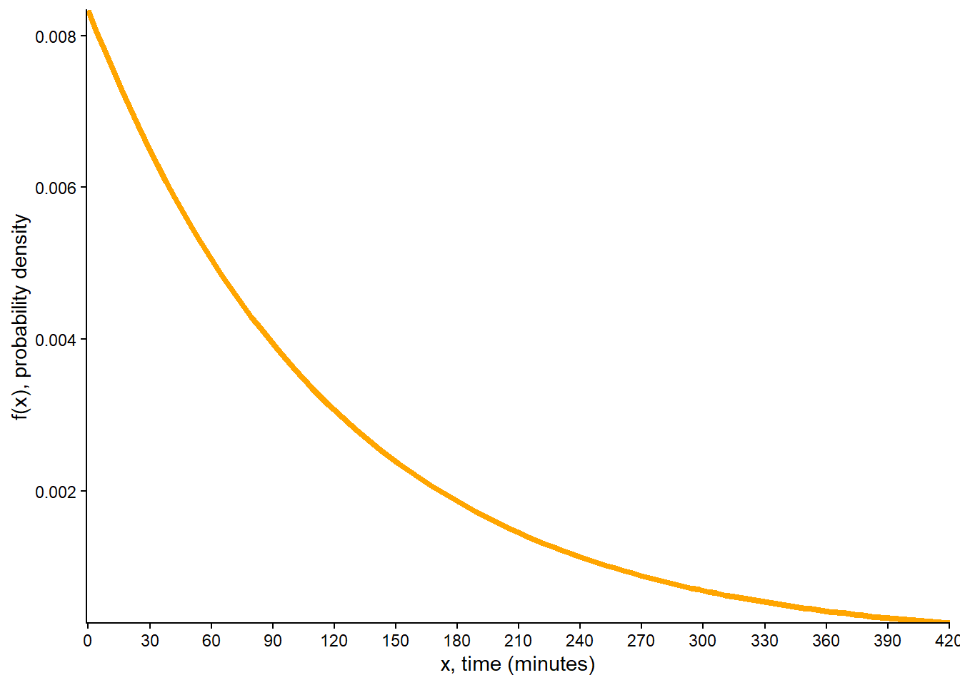
Example 7.15 This example is related to Example 5.6. Figure 5.10 suggests a form for the pdf.

Let \(X\) be the time (minutes) until the next earthquake occurs (of any magnitude in a certain region). Assume that the pdf of \(X\) is \[ f_X(x) = (1/120) e^{-x/120}, \qquad x \ge0 \]

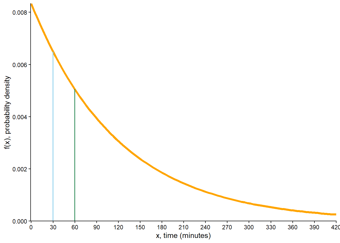
1. Sketch the pdf of \(X\) and verify that it resembles the orange curve in Figure 5.10.

2. Verify that \(f_X\) is a valid pdf.

3. Without doing any integration, approximate the probability that \(X\) rounded to the nearest second is 30 minutes.

4. Without doing any integration determine how much more likely that \(X\) rounded to the nearest second is to be 30 than 60 minutes.

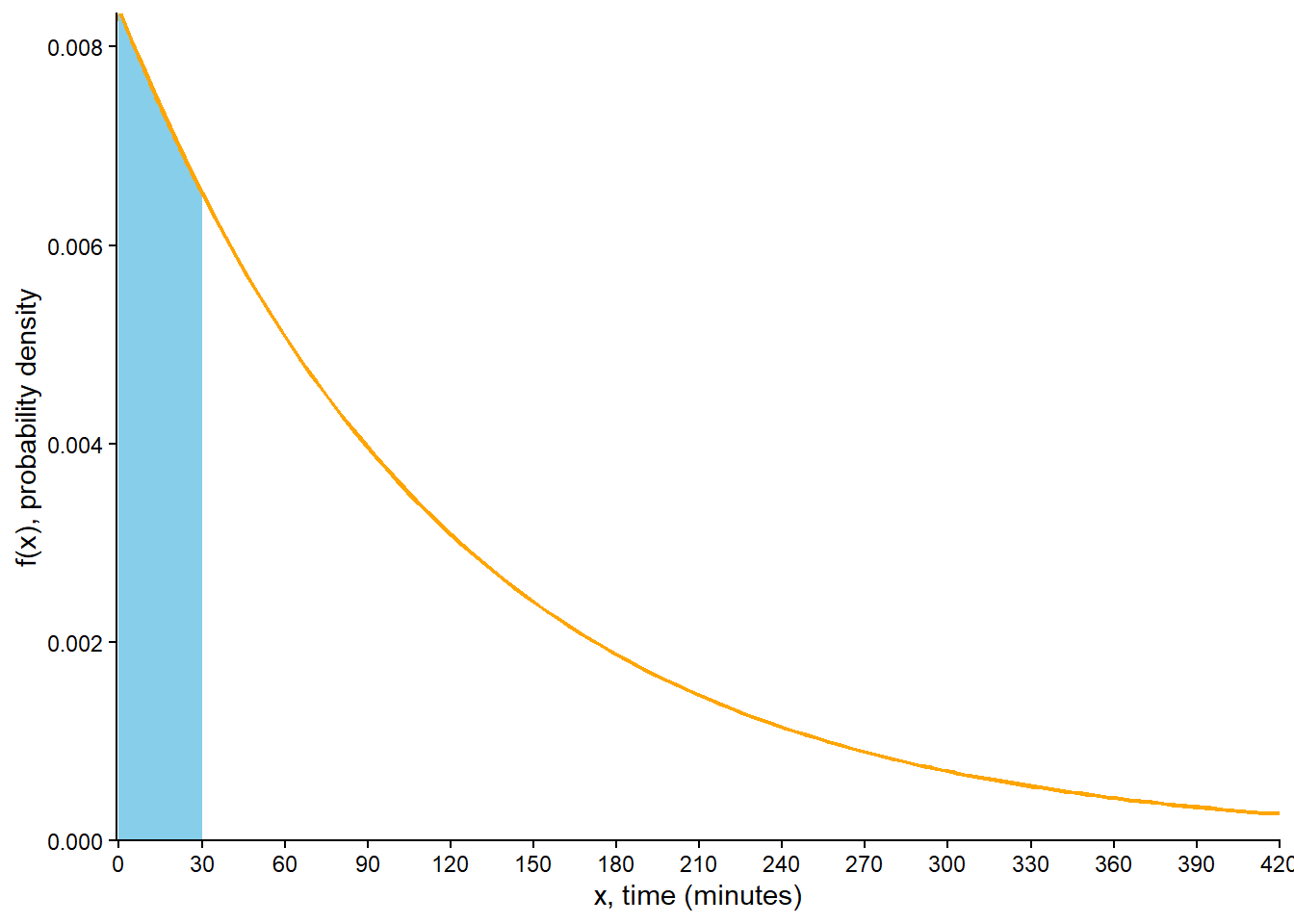
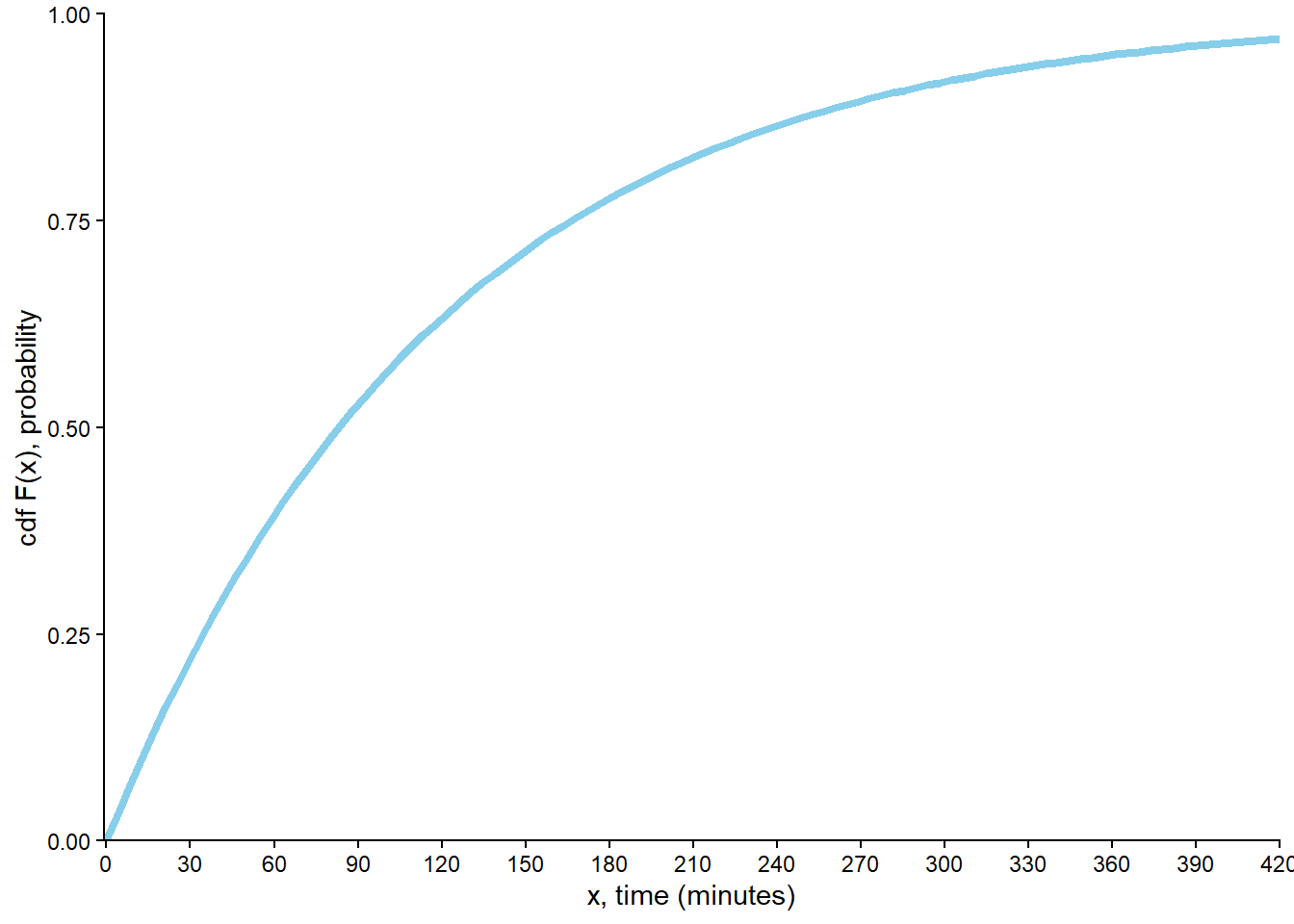
5. Compute and interpret \(\text{P}(X < 30)\).

6. Compute and interpret \(\text{P}(X > 360)\).

7. Find the cdf of \(X\).

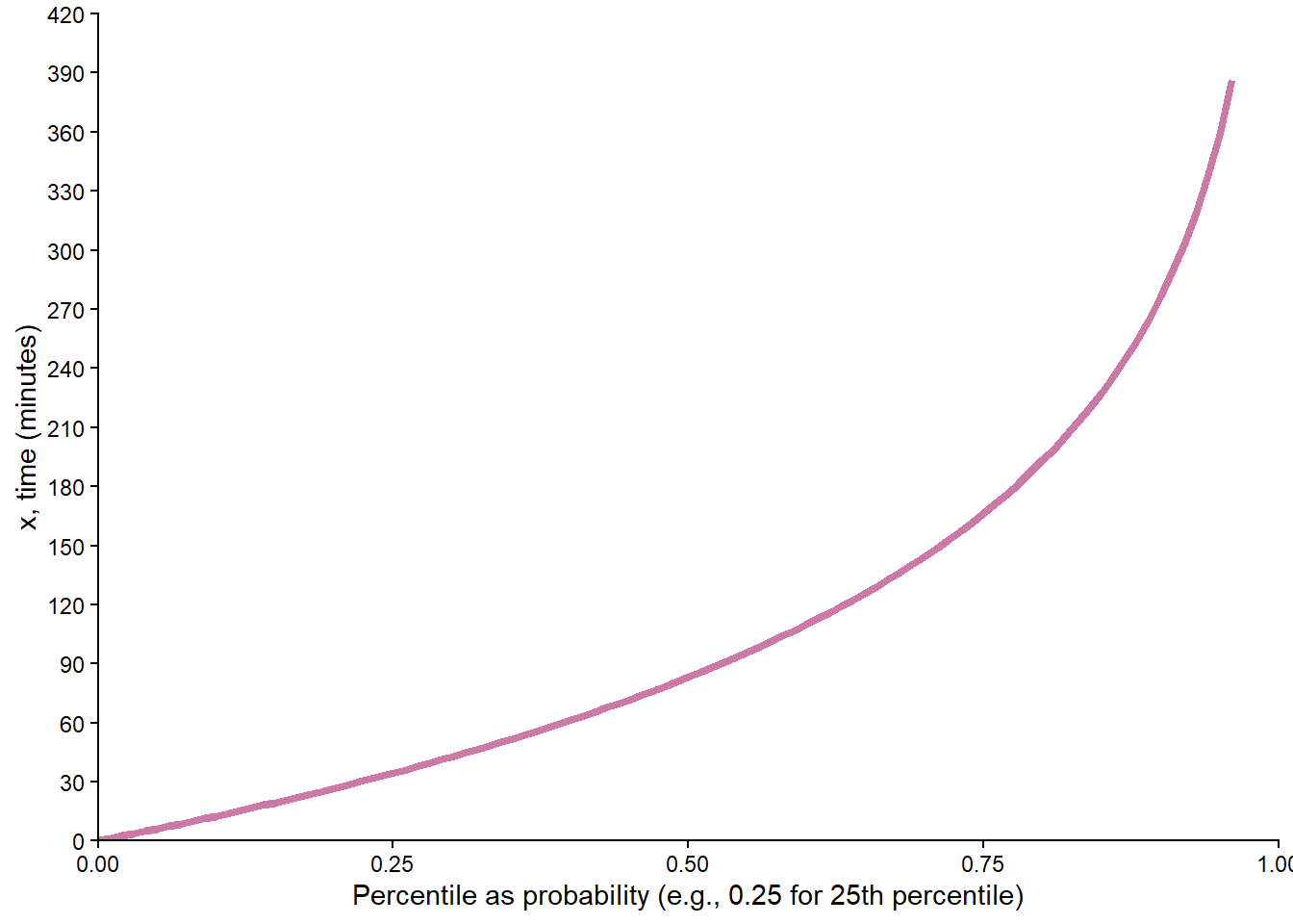
8. Find the 25th percentile of \(X\).

9. Find the quantile function of \(X\).

10. Verify that the cdf and quantile function are consistent with Table 5.1 and the spinner in Figure 5.9

Solution (click to expand)

Solution 7.15.

1. See Figure 7.2 (a). This is the same curve as in Figure 5.10.

2. We need to check that the total area under the curve, over the entire range of possible values \(x>0\), is 1 \[ \int_0^\infty (1/120) e^{-x/120} dx = 1 \]

3. We can approximate the probability with the area of a rectangle with base 1/60 minute (1 second) and height \(f(30)\). The approximate probability is \((1/60)f(60) = (1/60)(1/120 e^{-30/120}) = 0.000108\).

4. See Figure 7.2 (f). The ratio of the density heights is \(\frac{f(30)}{f(60)} = \frac{(1/120)e^{-30/120}}{(1/120)e^{-60/120}} =1.28\), so \(X\) rounded to the nearest second is 1.28 times more likely to be 30 than 60 minutes. Note that this ratio does not depend on how closely we’re rounding, as long as it’s small in the scale of the variable.

5. This probability is represented by the shaded area in Figure 7.2 (a). Integrate the pdf over [0, 30] \[ F(30) = \textrm{P}(X \le 30) = \int_0^{30} (1/120) e^{-x/120} dx = 1 - e^{-30/120} = 0.221 \] Over many earthquakes, less than 30 minutes elapse until the next earthquake for 22.1% of earthquakes.

6. Even though there is technically no upper bound on the possible values of \(X\), the probability that \(X\) exceeds 360 minutes is fairly small. \[ \int_{360}^\infty (1/120) e^{-x/120} dx = e^{-360/120} = 0.0498 \] Over many earthquakes, the elapses until the next earthquake exceeds 360 minutes for only about 5% of earthquakes.

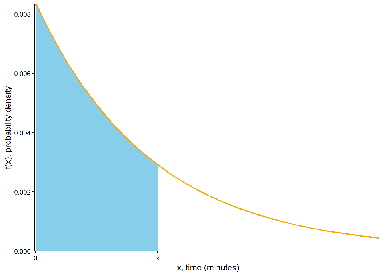
7. Repeat the calculation two parts above with 30 replaced by a generic \(x>0\). (Be careful with notation; since \(x\) is in the bounds we need a different dummy variable.) \[ F(x) = \textrm{P}(X \le x) = \int_0^{x} (1/120) e^{-u/120} du = 1 - e^{-x/120} \] For a given \(x>0\) this probability is represented by the area in Figure 7.2 (c). Technically the cdf is defined for all real values, so \[ F(x) = \begin{cases} 1-e^{-x/120}, & x>0,\\ 0, & x\le 0 \end{cases} \] See Figure 7.2 (d). Notice that the cdf is steepest, so probability accumulates more quickly, when the pdf is highest.

8. Set \(0.25 = F(x) = \textrm{P}(X \le x) = 1-e^{-x/120}\) and solve for \(x=-120\ln(1-0.25) = 34.5\) minutes.

9. Repeat the previous part with 0.25 replaced by a generic \(p\) between 0 and 1. Set \(p = F(x) = \textrm{P}(X \le x) = 1-e^{-x/120}\) and solve for \(x=-120\ln(1-p)\). The quantile function is \(Q(p) = -120\ln(1-p), 0<p<1\). See Figure 7.2 (e).

10. Plugging in a few values to \(F(x)\) shows that the cdf is consistent with Table 5.1; for example, \(F(42.8) = 1-e^{-42.8/120} = 0.3\), so 42.8 minutes is the 30th percentile. Plugging in a few values to \(Q(p)\) shows that the quantile funciton is consistent with Table 5.1; for example, \(Q(0.7) = -120\ln(1-0.7) = 144.5\), so 144.5 minutes is the 70th percentile. The spinner in Figure 5.9 can be used to simulate values of a random variable with this pdf.

(a) Probability density function

(b) Shaded area represents \(F(30)= \textrm{P}(X\le 30)\)

(c) Shaded area represents \(F(x)= \textrm{P}(X\le x)\)

(d) Cumulative distribution function

(e) Quantile function

(f) Comparison of \(f(30)\) and \(f(60)\)

Figure 7.2: Illustrations of Example 7.15

Starting with a pdf, we integrate to get the cdf.

Lemma 7.2 If \(X\) is a continuous random variable with pdf \(f_X\), its cdf \(F_X\) satisfies \[ F_X(x) = \int_{-\infty}^x f_X(u) du \]

A pdf must be integrated to compute probabilities. Think of the cdf as a generic integral. Rather than integrating separately to find \(F(30)\), \(F(60)\), etc, we integrate once with a generic \(x\) to find the general expression of the cdf \(F(x)\), then we can simplify plug in values to the cdf to compute probabilities.

Example 7.16 Recall Example 2.33. We started by assuming the cdf of \(X\) is \(F(x) = (x/60)^2, 0<x<60\). Use calculus to find the pdf. Compare to Example 5.11.

Solution (click to expand)

Solution 7.16. Since we integrate the pdf to get the cdf, we differentiate the cdf to get the pdf. For \(0<x<60\) \[ f(x) = \frac{d}{dx} (x/60)^2 = (2/3600) x, \] For \(x<0\), the cdf is constant (0), so the derivative is 0. For \(x>60\), the cdf is constant (1), so the derivative is 0. So the pdf of \(X\) is \[ f_X(x) = \begin{cases} (2/3600)x, & 0<x<60,\\ 0 & \text{otherwise.} \end{cases} \] which is the same as in Example 5.11.

Lemma 7.3 If \(X\) is a continuous random variable with cdf \(F_X\), its pdf \(f_X\) satisfies \[ f_X(x) = \frac{d}{dx} F_X(x) \]

7.7 Expected values of continuous random variables

An expected value is a probability-weighted average value. For a discrete random variable we multiply each possible value by its corresponding probability, determined by the pmf, and then sum. We can find the probability-weighted average value for continuous random variables analogously: multiply each possible value by its corresponding density, determined by the pdf, and then integrate.

Example 7.17 Suppose that \(X\) is a random variable with pdf \[ f_X(x) = e^{-x}, \qquad x \ge0 \]

1. Explain how you could use simulation to approximate \(\textrm{E}(X)\).

2. Suppose the values of \(X\) are truncated³ to integers. That is, 0.738 is recorded as 0, 1.154 is recorded as 1, 2.999 is recorded as 2, 3.001 is recorded as 3, etc. Table 7.10 summarizes 10000 simulated values of \(X\), truncated. Using just these values, approximate \(\textrm{E}(X)\).

3. How could you approximate the probability that the truncated value of \(X\) is 0? 1? 2? Suggest a formula for the approximate \(\textrm{E}(X)\). (Don’t worry if the approximation isn’t great; we’ll see how to improve it.)

4. Truncating to the nearest integer turns out not to yield a great approximation of the long run average value of \(X\). How could we get a better approximation?

5. Suppose instead of truncating to an integer, we truncate to the first decimal. For example 0.738 is recorded as 0.7, 1.154 is recorded as 1.1, 2.999 is recorded as 2.9, 3.001 is recorded as 3.0, etc. Suggest a formula for the approximate \(\textrm{E}(X)\).

6. Suppose instead of truncating to an integer, we truncate to the second decimal. For example 0.738 is recorded as 0.73, 1.154 is recorded as 1.15, 2.999 is recorded as 2.99, 3.001 is recorded as 3.00, etc. Suggest a formula for the approximate \(\textrm{E}(X)\).

7. We can continue in this way, truncating to the second decimal place, then the third, and so on. Considering what happens in the limit, suggest a formula for the theoretical \(\textrm{E}(X)\).

8. Donny Dont says \(\text{E}(X) = \int_0^\infty e^{-x}dx = 1\). Do you agree?

Table 7.10: 10000 simulated values of X, truncated, for X with an Exponential(1) distribution

10000 simulated values of X, truncated, for X with an Exponential(1) distribution

Truncated value of X	Number of repetitions
0	6302
1	2327
2	915
3	287
4	94
5	43
6	22
7	5
8	4
9	1

Solution (click to expand)

Example 7.18  

1. Simulate many values of \(X\) and average: sum the simulated values and divide by the number of simulated values. You can always approximate \(\textrm{E}(X)\) by simulating many values and averaging; it doesn’t matter if the random variable is discrete or continuous.

2. The truncated random variable is a discrete random variable, so we can compute the probability-weighted average as usual \[ 0\left(\frac{6302}{10000}\right)+ 1\left(\frac{2327}{10000}\right)+2\left(\frac{915}{10000}\right) + 3\left(\frac{287}{10000}\right)+ \cdots + 9\left(\frac{1}{10000}\right) \]

3. If \(X\) is between 0 and 1 then the truncated value is 1. We could find the probability that \(X\) is between 0 and 1 by integrating the pdf over this range. But we can approximate the probability by multiplying the pdf evaluated at 0.5 (the midpoint⁴) by the length of the (0, 1) interval: \(f(0.5)(1-0) = e^{-0.5}(1)\approx 0.607\). Technically, the approximation is not great unless the interval is short, but it’s the idea that is important for now. Similarly the approximate probability that the truncated value is 1 is \(f(1.5)(2-1) = e^{-1.5}(1)\approx 0.223\), and the approximate probability that the truncated value is 2 is \(f(2.5)(3-2) = e^{-2.5}(1)\approx 0.082\). Following this pattern, a reasonable formula for the truncated-to-nearest-integer discrete approximation of \(\textrm{E}(X)\) seems to be \[\begin{align*} & \qquad 0\left(f(0+ 0.5)(1)\right)+ 1\left(f(1 + 0.5)(1)\right)+2\left(f(2+0.5)(1)\right) + 3\left(f(3 + 0.5)(1)\right) + \cdots \\ & = \sum_{x=0}^\infty x f(x + 0.5) (1)\\ & = \sum_{x=0}^\infty x e^{-(x + 0.5)} (1) \end{align*}\] where the sum is over values \(x = 0, 1, 2, \ldots\). Plugging in \(f(x + 0.5) = e^{-(x+0.5)}\) to the above yields 0.558. This turns out to be a bad approximation, but the following part refine it.

4. Rather than truncating to integers, truncate to the first decimal, or the second, or the third. Or better yet don’t truncate; \(X\) is continuous after all. But it helps to consider what would happen if \(X\) were discrete first.

5. Now the possible values would be 0, 0.1, 0.2, etc. The truncated value would be 0 if \(X\) lies in the interval (0, 0.1). We could approximate this probability with \(f(0.05)(0.1-0) = e^{-0.05}(0.1)\). We could approximate the probability that \(X\) lies in the interval (0.1, 0.2), so the truncated value is 0.1, with \(f(0.15)(0.2-0.1) = e^{-0.15}(0.1)\). Following this pattern, a reasonable formula for the truncated-to-nearest-tenth discrete approximation of \(\textrm{E}(X)\) seems to be \[\begin{align*} & \qquad 0\left(f(0+ 0.05)(0.1)\right)+ 0.1\left(f(0.1 + 0.05)(0.1)\right)+0.2\left(f(0.2+0.05)(0.1)\right) + 0.3\left(f(0.3 + 0.05)(0.1)\right) + \cdots \\ & = \sum_{x=0}^\infty x f(x + 0.05) (0.1)\\ & = \sum_{x=0}^\infty x e^{-(x + 0.05)} (0.1) \end{align*}\] where the sum is over values \(x = 0, 0.1, 0.2, \ldots\). Plugging in \(f(x + 0.5) = e^{-(x+0.5)}\) to the above yields 0.950.

6. Truncating to the second decimal place suggests a formula for the long run average of \[\begin{align*} & \qquad 0\left(f(0+ 0.005)(0.01)\right)+ 0.01\left(f(0.01 + 0.005)(0.01)\right)+0.02\left(f(0.02+0.005)(0.01)\right) + 0.03\left(f(0.03 + 0.005)(0.01)\right) + \cdots \\ & = \sum_{x=0}^\infty x f(x + 0.005) (0.01)\\ & = \sum_{x=0}^\infty x e^{-(x + 0.005)} (0.01) \end{align*}\] where the sum is over values \(x = 0, 0.01, 0.02, \ldots\).
   Plugging in \(f(x) = e^{-x}\) to the above yields 0.995.

7. If \(\Delta x\) represents the level of truncation, e.g., \(\Delta x = 0.01\) for truncating to the second decimal place, then a general formula is \[\begin{align*} & \qquad \sum_{x=0}^\infty x f(x + \Delta x / 2) \Delta x\\ & = \sum_{x=0}^\infty x e^{-x + \Delta x / 2} \Delta x\\ & \approx \sum_{x=0}^\infty x e^{-x} \Delta x \end{align*}\] In the limit as \(\Delta x\) approaches 0, \(f(x + \Delta x /2)\) approaches \(f(x)=e^{-x}\), there are more and more terms in the sum, and the sum approaches an integral over \(x\) values, \[\begin{align*} & \qquad \int_0^\infty x f(x) dx\\ & = \int_0^\infty x e^{-x} dx \end{align*}\]

8. Donny happened to get the correct value, but that’s just coincidence. His method is wrong. Donny integrated the pdf over the range of all possible values, \(\int_0^\infty f_X(x)dx\), which will always be 1. To get the expected value, you need to find the probability weighted average value of \(x\): \(\int_0^\infty x f_X(x)dx\).

Definition 7.6 Let \(X\) be a continuous random variable with pdf \(f_X\). The expected value of \(X\) is \[ \textrm{E}(X) = \int_{-\infty}^\infty x f_X(x) dx \]

Remember to replace the generic bounds \((\infty, \infty)\) with the range of possible values of \(X\).

Warning

Remember that an expected value is a probaility-weighted average: take each possible value of the variable and multiply by its probability. For a continuous random variable \(X\) with pdf \(f_X\) the calculation is \(\int_{-\infty}^\infty x f_X(x)dx\). In \(x f_X(x)\) the first \(x\) plays the role of “value” and \(f_X(x)\) plays the role of “probability”. The pdf \(f_X(x)\) might be a fairly complicated function of \(x\), so it’s easy to lose the \(x\) out front. But don’t forget that \(x\)! Omitting the \(x\) gives \(\int_{-\infty}^\infty f_X(x)dx\) which will always be 1 since it’s the integral of a pdf. Anytime you compute an expected value and it turns out to be 1, be a little suspicious and double check that you didn’t forget the \(x\) that multiplies \(f_X(x)\).

Example 7.19 Continuing Example 7.15. Let \(X\) be the times (minutes) until the next earthquake occurs (of any magnitude in a certain region). Assume that the pdf of \(X\) is \[ f_X(x) = (1/120) e^{-x/120}, \qquad x \ge0 \]

1. Donny Dont says \(\text{E}(X) = \int_0^\infty (1/120)e^{-x/120}dx = 1\). Do you agree?

2. Compute and interpret \(\text{E}(X)\).

3. Compute and interpret \(\text{P}(X \le \text{E}(X))\).

Solution (click to expand)

Solution 7.17.

1. Donny didn’t heed the previous warning; he forgot to multiply the pdf by \(x\) so he is just integrating the pdf which yields 1.

2. \(\text{E}(X) = \int_0^\infty x f_X(x)dx = \int_0^\infty x (1/120)e^{-x/120} = 120\) minutes. Over many earthquakes, the elapsed time between earthquakes is 120 minutes on average.

3. The cdf is \(F(x) = 1 - e^{-x/120}\), so \[ \textrm{P}(X \le \textrm{E}(X)) = \textrm{P}(X \le 120) = F(120) = 1-e^{-120/120} = 1-e^{-1} = 0.632 \] In this case, the mean 120 is greater that the median of 83 minutes. The distribution is skewed to the right, so the longer tail representing the distribution of larger values pulls the mean up.

Lemma 7.4 (Law of the unconscious statistician (LOTUS)) If \(X\) is a continuous random variable with pdf \(f_X\) and \(g\) is any function, \[ \textrm{E}[g(X)] =\int_{-\infty}^\infty g(x) f_X(x) dx \]

LOTUS says we don’t have to first find the distribution of \(Y=g(X)\) to find \(\textrm{E}[g(X)]\); rather, we just simply apply the transformation \(g\) to each possible value \(x\) of \(X\) and then apply the corresponding weight for \(x\) to \(g(x)\).

Recall that whether in the short run or the long run, in general \[\begin{align*} \text{Average of $g(X)$} & \neq g(\text{Average of $X$}) \end{align*}\] In terms of expected values, in general \[\begin{align*} \text{E}(g(X)) & \neq g(\text{E}(X)) \end{align*}\] The left side \(\text{E}(g(X))\) represents first transforming the \(X\) values and then averaging the transformed values. The right side \(g(\text{E}(X))\) represents first averaging the \(X\) values and then plugging the average (a single number) into the transformation formula.

Example 7.20 Continuing Example 7.19. Let \(X\) be the times (minutes) until the next earthquake occurs (of any magnitude in a certain region). Assume that the pdf of \(X\) is \[ f_X(x) = (1/120) e^{-x/120}, \qquad x \ge0 \] We’re interested in \(\textrm{E}(X^2)\) and \(\textrm{Var}(X)\).

1. Donny Dont says: “I can just use LOTUS and replace \(x\) with \(x^2\), so \(\text{E}(X^2)\) is \(\int_{-\infty}^{\infty} (1/120)x^2 e^{-x^2/120} dx\)”. Do you agree?

2. Compute \(\text{E}(X^2)\).

3. Compute \(\text{Var}(X)\).

4. Compute \(\text{SD}(X)\).

Solution (click to expand)

Solution 7.18.

1. The point of LOTUS is that we transform the values of \(X\) but not the probabilities. That is, the pdf of \(X\), \(f_X(x) = (1/120)e^{-x/120}\) is unchanged.

2. \(\textrm{E}(X^2) = \int_0^\infty x^2 f_X(x) dx = \int_0^\infty x^2 (1/120)e^{-x/120} dx = 28800\) squared-minutes.

3. \(\text{Var}(X) = \textrm{E}(X^2) - (\textrm{E}(X))^2 = 28800 - 120^2 = 14400\) squared-minutes.

4. \(\text{SD}(X)=\sqrt{\textrm{Var}(X)} = \sqrt{14400} = 120\) minutes.

7.8 Exponential distributions

Exponential distributions are often used as models for random variables which measure the times between events in the random process that happens over time. We have already seen several examples of Exponential distributions, including Example 7.15 and Example 7.18.

Definition 7.7 A continuous random variable \(X\) has an Exponential distribution with rate parameter \(\lambda>0\) if and only if its probability density function \(f_X\) satisfies \[ f_X(x) = \begin{cases} \lambda e^{-\lambda x}, & x \ge 0,\\ 0, & \text{otherwise} \end{cases} \] Equivalently, a continuous random variable \(X\) has an Exponential distribution with rate parameter \(\lambda>0\) if and only if its cumulative distribution function \(F_X\) satisfies \[ F_X(x) = \begin{cases} 1- e^{-\lambda x}, & x \ge 0,\\ 0, & \text{otherwise} \end{cases} \]

Lemma 7.5 If \(X\) has an Exponential distribution with rate parameter \(\lambda>0\) then \[\begin{align*} \text{P}(X>x) & = e^{-\lambda x}, \quad x\ge 0\\ \text{quantile:} \quad Q(p) & = -(1/\lambda) \ln(1-p),\quad 0<p<1\\ \text{E}(X) & = \frac{1}{\lambda}\\ \text{Var}(X) & = \frac{1}{\lambda^2}\\ \text{SD}(X) & = \frac{1}{\lambda} \end{align*}\]

Warning

The parameter \(\lambda\) in our definition of Exponential distributions is the rate parameter, so that the mean is \(1/\lambda\). Other references might parameterize Exponential distributions in terms of their mean. When dealing with problems involving Exponential distributions pay close attention to whether the rate (\(\lambda\)) or the mean (\(1/\lambda\)) is specified.

7.9 Normal distributions

Normal distributions are probably the most important distributions in probability and statistics. We have already seen Normal distributions in many previous examples. In this section we’ll explore mathematical properties of Normal distributions in a little more depth.

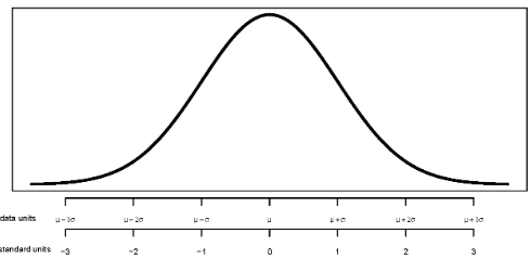
Recall Section 5.10, Figure 5.22, and Table 5.5. Any Normal distribution follows the “empirical rule” which specifies a specific pattern of percentiles in terms of standard deviations from the mean and gives a Normal pdf its particular bell-shape. Now we’ll look more closely at the mathematical expression of a Normal pdf.

A Normal density is a continuous density on the real line with a particular symmetric “bell” shape. The heart of a Normal pdf is the function \[ e^{-z^2/2}, \qquad -\infty < z< \infty, \] which defines the general shape of a Normal density. It can be shown that \[ \int_{-\infty}^\infty e^{-z^2/2}dz = \sqrt{2\pi} \] Therefore the function \(e^{-z^2/2}/\sqrt{2\pi}\) integrates to 1.

Definition 7.8 A continuous random variable \(Z\) has a Standard Normal distribution if its pdf⁵ is \[ \phi(z) = \frac{1}{\sqrt{2\pi}}\,e^{-z^2/2}, \quad -\infty<z<\infty \]

Z = RV(Normal())

Z.sim(100).plot('rug')
plt.show()

z = Z.sim(10000)

z.plot()

Normal().plot()

<symbulate.distributions.Normal object at 0x0000027B7A3C4550>

plt.show()

z.mean(), z.sd()

(0.013822039345898478, 1.00156299489968)

If \(Z\) has a Standard Normal distribution then

\[\begin{align*} \textrm{E}(Z) & = 0\\ \textrm{SD}(Z) & = 1 \end{align*}\]

The Standard Normal pdf is symmetric about its mean of 0, and the peak of the density occurs at 0. The standard deviation is 1, and 1 also indicates the distance from the mean to where the concavity of the density changes. That is, there are inflection points at \(\pm1\).

A random variable with a Standard Normal distribution is in standardized units; the mean is 0 and the standard deviation is 1. We can obtain Normal distribution with other means and standard deviations via linear rescaling. If \(Z\) has a Standard Normal distribution then \(X=\mu + \sigma Z\) has a Normal distribution with mean \(\mu\) and standard deviation \(\sigma\). The linear transformation does not change the shape; \(X\) will have a Normal distribution. Adding the constant \(\mu\) shifts the center so that \(\textrm{E}(X)=\mu\). Multiplying by the constant \(\sigma\) changes the scale so that \(\textrm{SD}(X)=\sigma\). Since the scale is changed, the density heights must also be revised so that the total area under the curve remains 1.

Definition 7.9 A continuous random variable \(X\) has a Normal (a.k.a., Gaussian) distribution with mean \(\mu\in (-\infty,\infty)\) and standard deviation \(\sigma>0\) if its pdf is \[ f_X(x) = \frac{1}{\sigma\sqrt{2\pi}}\,\exp\left(-\frac{1}{2}\left(\frac{x-\mu}{\sigma}\right)^2\right), \quad -\infty<x<\infty. \]

Figure 7.3: A generic Normal pdf.

If \(X\) has a Normal(\(\mu\), \(\sigma\)) distribution then⁶ \[\begin{align*} \textrm{E}(X) & = \mu\\ \textrm{SD}(X) & = \sigma \end{align*}\]

A Normal density is a particular “bell-shaped” curve which is symmetric about its mean \(\mu\). The mean \(\mu\) is a location parameter: \(\mu\) indicates where the center and peak of the distribution is.

The standard deviation \(\sigma\) is a scale parameter: \(\sigma\) indicates the distance from the mean to where the concavity of the density changes. That is, there are inflection points at \(\mu\pm \sigma\).

Example 7.21 The pdfs in the plot below represent the distribution of hypothetical test scores in three classes. The test scores in each class follow a Normal distribution. Identify the mean and standard deviation for each class.

<symbulate.distributions.Normal object at 0x0000027B7AB6CA50>

<symbulate.distributions.Normal object at 0x0000027B7916DA70>

<symbulate.distributions.Normal object at 0x0000027B7916E520>

Solution (click to expand)

Solution 7.19. The blue curve corresponds to a mean of 60; the others to a mean of 70. The green curve corresponds to a standard deviation of 5. Notice that the concavity changes around 65 and 75, so 5 is the distance from the mean to the inflection points. The standard deviation is 10 in the other plots. The total area under each curve is 1.

If \(Z\) has a Standard Normal distribution its cdf is \[ \Phi(z) = \textrm{P}(Z \le z) = \int_{-\infty}^z \frac{1}{\sqrt{2\pi}}\,e^{-u^2/2}du, \quad -\infty<z<\infty. \] However, there is no closed-form expression for the above integral. The above integral, hence probabilities for a Standard Normal distribution, must be computed through numerical methods. See Figure 5.22 and Table 5.5.

(a) Normal(0, 1) pdf \(\phi(z)\); shaded area represents \(\Phi(-0.67) = 0.25\)

(b) Normal(0, 1) cdf \(\Phi(z)\); \(\Phi(-0.67) = 0.25\) is highlighted

(c) spinner; shaded area represents \(\Phi(-0.67) = 0.25\)

Figure 7.4: Standard Normal distribution.

If \(X\) has a Normal(\(\mu\), \(\sigma\)) distribution then \(X\) has the same distribution as \(\mu + \sigma Z\) where \(Z\) has a Standard Normal distribution, so its cdf is \[ F_X(x) = \textrm{P}(X \le x) = \textrm{P}(\mu + \sigma Z \le x) = \textrm{P}\left(Z \le \frac{x-\mu}{\sigma}\right) = \Phi\left(\frac{x-\mu}{\sigma}\right) \] Therefore, probabilities for any Normal distribution can be found by standardizing and using the Standard Normal cdf, which is basically what we do when we use the “empirical rule”. See Figure 5.22 and Table 5.5.

Example 7.22 Use the empirical rule to evaluate the following.

1. \(\Phi(-1)\)
2. \(\Phi(1.5)\)
3. \(\Phi^{-1}(0.31)\)
4. \(\Phi^{-1}(0.975)\)

Solution (click to expand)

Solution 7.20. We could use a Normal distribution calculator, or we could just use Table 5.5.

1. \(\Phi(-1)\approx 0.16\).
2. \(\Phi(1.5)\approx 0.935\).
3. \(\Phi^{-1}(0.31)\approx -0.5\). The inverse of the cdf is the quantile function; \(\Phi^{-1}(0.31)\) represents the 31st percentile.
4. \(\Phi^{-1}(0.975)\approx 2\). The inverse of the cdf is the quantile function; \(\Phi^{-1}(0.975)\) represents the 97.5th percentile.

Normal().cdf(-1), Normal().cdf(1.5)

(np.float64(0.15865525393145707), np.float64(0.9331927987311419))

Normal().quantile(0.31), Normal().quantile(0.975)

(np.float64(-0.4958503473474533), np.float64(1.959963984540054))

Probabilities and quantiles for Normal distributions can be computed with software. However, you should practice making ballpark estimates without software, by standardizing and using the empirical rule.

Standardization is a specific linear rescaling. If \(X\) has a Normal distribution then any linear rescaling of \(X\) also has a Normal distribution.
Namely, if \(X\) has a Normal\(\left(\mu,\sigma\right)\) distribution and \(Y=aX+b\) for constants \(a,b\) with \(a\neq 0\), then \(Y\) has a Normal\(\left(a\mu+b, |a|\sigma\right)\) distribution.

Any linear combination of independent Normal random variables has a Normal distribution. If \(X\) and \(Y\) are independent, each with a marginal Normal distribution, and \(a, b\) are non-random constants then \(aX + bY\) has a Normal distribution. (We will see a more general result when we discuss Bivariate Normal distributions.)

Example 7.23 Two people are meeting. (Who? You decide!) Arrival time are measured in minutes after noon, with negative times representing arrivals before noon. Each arrival time follows a Normal distribution with mean 30 and SD 17 minutes, independently of each other.

1. Compute the probability that the first person to arrive has to wait more than 15 minutes for the second person to arrive.

2. Compute the probability that the first person to arrive arrives before 12:15.

Solution (click to expand)

Solution 7.21.

1. Let \(X, Y\) be the two arrival times, so that \(W=|X-Y|\) is the waiting time. We want \(\text{P}(|X - Y| >15) = \text{P}(X - Y > 15) + \text{P}(X - Y < -15)\). Since \(X\) and \(Y\) are independent each with a Normal distribution, then \(X - Y\) has a Normal distribution; the mean is \(30-30 = 0\), and since \(X\) and \(Y\) are independent \[ \text{Var}(X - Y) = \text{Var}(X) + \text{Var}(V) - 2\text{Cov}(X, Y) = 17^2 + 17^2 - 0 = 578 \] So \(\text{SD}(X - Y) = \sqrt{578} = 24.0\). The standardized value for 15 is \((15 - 0)/24.0=0.624\); that is, 15 is 0.624 SDs above the mean, so \(\textrm{P}(X - Y>15) = 0.266\). Since the distribution of \(X - Y\) is symmetric about 0, \[ \textrm{P}(W > 15) = \textrm{P}(|X-Y|>15) = \textrm{P}(X - Y > 15) + \textrm{P}(X - Y < - 15) = 2(0.266) = 0.53. \] On about 53% of days the first person to arrive has to wait more than 15 minutes for the second to arrive.

2. \(T = \min(X, Y)\) is the time at which the first person arrives. The first person arrives before 12:15 if either \(X<15\) or \(Y < 15\), so \(\textrm{P}(T < 15) = \textrm{P}(\{X < 15\}\cup\{Y < 15\})\). It’s easier to compute the probability of the complement. Note that 15 is 0.88 SDs below the mean of \(X\) (\((15 - 30)/17 = -0.88\)) so \(\textrm{P}(X>15) = 0.811\); similarly, \(\textrm{P}(Y > 15) = 0.811\). We want \[\begin{align*} \textrm{P}(T < 15) & = 1 - \textrm{P}(X > 15, Y > 15) && \text{Complement rule}\\ & = 1 - \textrm{P}(X>15)\textrm{P}(Y > 15) && \text{independence of $X, Y$}\\ & = 1- (0.811)(0.811) & & \text{Normal distributions}\\ & = 0.342 \end{align*}\] On about 34% of days the first person arrives before 12:15.

X, Y = RV(Normal(mean = 30, sd = 17) * Normal(mean = 30, sd = 17))

W = abs(X - Y)

T = (X & Y).apply(min)

w = W.sim(10000)

plt.figure()
w.plot()
plt.show()

w.mean(), w.sd(), w.count_gt(15) / w.count()

(19.248483751164667, 14.583082801755694, 0.5333)

t = T.sim(10000)

plt.figure()
t.plot()
plt.show()

t.mean(), t.sd(), t.count_lt(15) / w.count()

(20.53331479290535, 14.03191683715439, 0.3374)

Example 7.24 Daily high temperatures (degrees Fahrenheit) in San Luis Obispo in August follow (approximately) a Normal distribution with a mean of 76.9 degrees F. The temperature exceeds 100 degrees Fahrenheit on about 1.5% of August days.

1. Compute the standard deviation.

2. Suppose the mean increases by 2 degrees Fahrenheit. On what percentage of August days will the daily high temperature exceed 100 degrees Fahrenheit? (Assume the standard deviation does not change.)

3. A mean of 78.9 is 1.02 times greater than a mean of 76.9. By what (multiplicative) factor has the percentage of 100-degree days increased? What do you notice?

Solution (click to expand)

Solution 7.22.

1. We are given that 100 is the 98.5th percentile. Software (Normal(0, 1).quantile(0.985)) shows that for a Normal distribution the 98.5th percentile is 2.17 standard deviations above the mean. Set \(100 = 76.9 + 2.17\sigma\) and solve for the standard deviation \(\sigma = 10.65\) degrees F.

2. The mean is now 78.9. Now the value 100 is \((100-78.9)/10.65 = 1.98\) standard deviations above the mean. Software (1 - Normal(0, 1).cdf(1.98)) shows that for a Normal distribution the probability of a value more than 1.98 standard deviations above the mean is 0.023. On 2.3% of August days the daily high temperature will exceed 100 degrees F.

3. \(0.023/0.015 = 1.53\). A 2 percent increase in the mean results in a 53 percent increase in the probability that a day has a daily high temperature above 100 degrees F. Relative small changes in the mean can have relative large impacts on tail probabilities.

Example 7.25 In a large class, scores on midterm 1 follow (approximately) a Normal\((\mu_1, \sigma)\) distribution and scores on midterm 2 follow (approximately) a Normal\((\mu_2, \sigma)\) distribution. Note that the SD \(\sigma\) is the same on both exams. The 40th percentile of midterm 1 scores is equal to the 70th percentile of midterm 2 scores. Compute and interpret \[ \frac{\mu_1-\mu_2}{\sigma} \] (This is one statistical measure of effect size.)

Solution (click to expand)

Example 7.26 Software shows that for a Normal distribution, the 40th percentile is 0.253 SDs below the mean and the 70th percentile is 0.524 SDs above the mean. The 40th percentile of midterm 1 scores is \(\mu_1 - 0.253 \sigma\), and the 70th percentile of midterm 2 scores is \(\mu_2 + 0.524\sigma\). We are told \[ \mu_1 - 0.253 \sigma = \mu_2 + 0.524\sigma \] Solve for \[ \frac{\mu_1-\mu_2}{\sigma} = 0.524 + 0.253 = 0.78 \] The effect size is 0.78. The mean on midterm 1 is 0.78 SDs above the mean on midterm 2.

The previous example illustrates a common problem in statistics: comparing two (or more) groups; in particular, comparing two means. When comparing groups, a more important question than “is there a difference?” is “how large is the difference?” An effect size is a measure of the magnitude of a difference between groups. When comparing a numerical variable between two groups, one measure of the population effect size is Cohens’s \(d\) \[ \frac{\mu_1 - \mu_2}{\sigma} \]

The values of any numerical variable vary naturally from unit to unit. The SD of the numerical variable measures the degree to which individual values of the variable vary naturally, so the SD provides a natural “scale” for the variable. Cohen’s \(d\) compares the magnitude of the difference in means relative to the natural scale (SD) for the variable

Some rough guidelines for interpreting \(|d|\):

d	0.2	0.5	0.8	1.2	2.0
Effect size	Small	Medium	Large	Very Large	Huge

For example, assume the two population distributions are Normal and the two population standard deviations are equal. Then when the effect size is 1.0 the median of the distribution with the higher mean is the 84th percentile of the distribution with the lower mean, which is a very large difference.

d	0.2	0.5	0.8	1.0	1.2	2.0
Effect size	Small	Medium	Large		Very Large	Huge
Median of population 1 is
(blank) percentile of population 2	58th	69th	79th	84th	89th	98th

---

1. There are easier proofs, e.g., using moment generating functions.

2. When there are \(n\) trials, the probability of success on each of the \(n\) trials is \(p_n\). The subscript \(n\) indicates that this value can change as \(n\) changes (e.g. 1/10 when \(n=10\), 1/100 when \(n=100\)), so that when \(n\) is large \(p\) is small enough to maintain relative “rarity”.

3. We could also round to the nearest integer. Whether we truncate or round won’t matter as we consider what happens in the limit.

4. In the limit, any value in (0, 1) would work. We use the midpoint mostly because just using using 0 results in an approximate probability of \(e^{-0}(1)=1\), an egregious approximation of the true probability \(1-e^{-1}\approx 0.632\)

5. The Standard Normal pdf is typically denoted \(\phi(\cdot)\), the lowercase Greek letter “phi”, and the cdf is denoted \(\Phi(\cdot)\), the uppercase Greek letter “phi”.

6. If we write \(N(0, 4)\) we mean a Normal distribution with mean 0 and standard deviation 4. Be aware that some references refer to a Normal distribution by its mean and variance, in which case \(N(0, 4)\) would refer to a Normal distribution with mean 0 and variance 4.