10 Chapter 3 Exercise Solutions
10.1 Solution to Exercise 3.1
Label 365 cards with the numbers 1 through 365. Shuffle the cards and deal \(n\) with replacement. If the \(n\) cards dealt all have different numbers, then \(B\) does not occur; otherwise \(B\) occurs.
10.2 Solution to Exercise 3.2
Create a spinner with two sectors, one sector labeled “make” which accounts for 40% of the area, and the other 60% labeled “miss”. Spinner the spinner until it lands on “make” and then stop; let \(X\) be the total number of spins.
10.3 Solution to Exercise 3.3
Create a spinner with three equal sectors, labeled 1, 2, 3. Spin the spinner 3 times. Let \(X\) be the number of distinct numbers the spinner lands on; for example if the spinner lands on 3 then 1 then 3, then \(X\) is 2. Let \(Y\) be the number of spins that land on 1.
10.4 Solution to Exercise 3.4
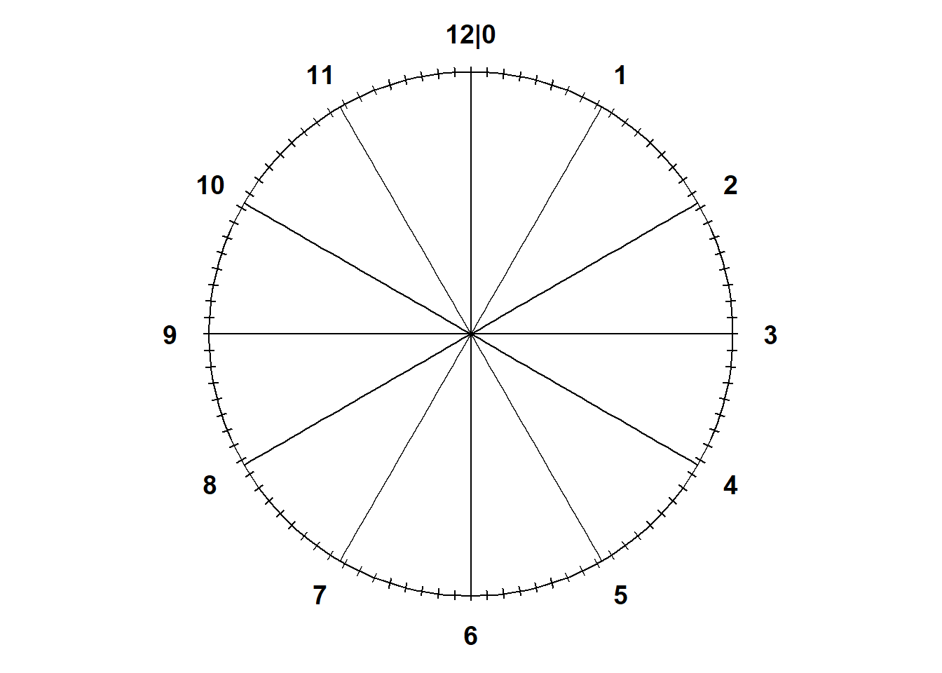
- A Uniform(0, 12) spinner is basically a clock. It goes from 0 to 12 in equally spaced increments. See Figure 10.1.
- To simulate \(X\), flip the coin to determine if the point is in the “east” or “west” and then spin the Uniform(0, 12) spinner to determine how far from the center in the east or west direction. Let the result of the spin be \(U_1\). If the coin lands on heads (east) set \(X=U_1\); if the coin lands on tails (west) set \(X=-U_1\). To simulate \(Y\), spin the spinner again to get \(U_2\), and flip the coin again. If the result of the flip is heads (north) then set \(Y = U_2\); if the result of the flip is tails (south) then set \(Y=-U_2\). Compute the distance from \((X, Y)\) to (0, 0) as \(R=\sqrt{X^2+Y^2}\). If \(R>12\) the dart would land off the board, so just discard the repetition and try again.
- Exercise 2.13 shows that \(R\) is not uniformly distributed between 0 and 12. In particular, \(R\) is more likely to be between 11 and 12 than it is to be between 0 and 1. Therefore a Uniform(0, 12) spinner would not be appropriate.
10.5 Solution to Exercise 3.5
10.6 Solution to Exercise 3.6
P = BoxModel([1, 2, 3], size = 3)

def count_distinct(u):
    return len(set(u))

X = RV(P, count_distinct)

Y = RV(P, count_eq(1))

(RV(P) & X & Y).sim(10)| Index | Result |
|---|---|
| 0 | ((2, 1, 3), 3, 1) |
| 1 | ((1, 2, 3), 3, 1) |
| 2 | ((1, 3, 3), 2, 1) |
| 3 | ((3, 2, 3), 2, 0) |
| 4 | ((1, 1, 2), 2, 2) |
| 5 | ((1, 3, 2), 3, 1) |
| 6 | ((1, 3, 1), 2, 2) |
| 7 | ((1, 3, 2), 3, 1) |
| 8 | ((3, 2, 2), 2, 0) |
| ... | ... |
| 9 | ((1, 1, 3), 2, 2) |
10.7 Solution to Exercise 3.7
P = BoxModel([1, 2, 3], size = 3, probs = [0.1, 0.3, 0.6])

def count_distinct(u):
    return len(set(u))

X = RV(P, count_distinct)

Y = RV(P, count_eq(1))

(RV(P) & X & Y).sim(10)| Index | Result |
|---|---|
| 0 | ((3, 3, 3), 1, 0) |
| 1 | ((3, 3, 2), 2, 0) |
| 2 | ((3, 3, 3), 1, 0) |
| 3 | ((3, 2, 2), 2, 0) |
| 4 | ((3, 3, 3), 1, 0) |
| 5 | ((1, 1, 1), 1, 3) |
| 6 | ((1, 2, 2), 2, 1) |
| 7 | ((2, 3, 2), 2, 0) |
| 8 | ((3, 3, 3), 1, 0) |
| ... | ... |
| 9 | ((3, 2, 3), 2, 0) |
10.8 Solution to Exercise 3.8
The code below defines a random variable \(X\) that counts the number of distinct birthdays in the group of \(n\). Event \(B\) occurs if \(X<n\).
n = 30

P = BoxModel(list(range(365)), size = n)

def count_distinct(u):
  return len(set(u))

X = RV(P, count_distinct)

B = (X < n)

B.sim(10)| Index | Result |
|---|---|
| 0 | False |
| 1 | False |
| 2 | True |
| 3 | False |
| 4 | True |
| 5 | False |
| 6 | True |
| 7 | True |
| 8 | True |
| ... | ... |
| 9 | True |
10.9 Solution to Exercise 3.9
p_success = 0.4

# define a function that takes as an input a sequence of 0s and 1s (omega)
# and returns when the first 1 occurs
def count_until_first_success(omega):
    for i, w in enumerate(omega):
        if w == 1:
            return i + 1 # the +1 is for zero-based indexing

# Either of the following probability spaces works
# P = Bernoulli(p_success) ** inf
P = BoxModel([1, 0], probs = [p_success, 1 - p_success], size = inf)

X = RV(P, count_until_first_success)

(RV(P) & X).sim(10)| Index | Result |
|---|---|
| 0 | ((1, 0, 0, 0, 0, 1, ...), 1) |
| 1 | ((0, 0, 0, 1, 0, 1, ...), 4) |
| 2 | ((0, 1, 0, 1, 0, 0, ...), 2) |
| 3 | ((0, 0, 0, 1, 0, 1, ...), 4) |
| 4 | ((1, 1, 1, 0, 0, 0, ...), 1) |
| 5 | ((0, 0, 0, 1, 1, 1, ...), 4) |
| 6 | ((0, 0, 0, 0, 1, 1, ...), 5) |
| 7 | ((1, 0, 0, 1, 1, 0, ...), 1) |
| 8 | ((0, 0, 0, 1, 0, 0, ...), 4) |
| ... | ... |
| 9 | ((1, 1, 0, 0, 0, 0, ...), 1) |
10.10 Solution to Exercise 3.10
In the code below
Uniform(0, 12) ** 2corresponds to the two spinsBoxModel([-1, 1], size = 2)corresponds to the two coin flipsUniform(0, 12) ** 2 * BoxModel([-1, 1], size = 2)simulates a pair which we unpack and define asRVsU, F, butUis itself a pair and so isF.U[0]is the first spin andF[0]is the first flip.
U, F = RV(Uniform(0, 12) ** 2 * BoxModel([-1, 1], size = 2))

X = U[0] * F[0]

Y = U[1] * F[1]

R = sqrt(X ** 2 + Y ** 2)

(U & F & X & Y & R).sim(10)| Index | Result |
|---|---|
| 0 | ((6.178279200148128, 2.1416667390135995), (1, -1), 6.178279200148128, -2.1416667390135995, 6.5389502... |
| 1 | ((10.59306795477702, 11.350115436070693), (1, 1), 10.59306795477702, 11.350115436070693, 15.52540527... |
| 2 | ((3.02452656952319, 6.9199924289044334), (-1, 1), -3.02452656952319, 6.9199924289044334, 7.552089524... |
| 3 | ((5.259827970982579, 3.144916384538416), (1, -1), 5.259827970982579, -3.144916384538416, 6.128318639... |
| 4 | ((7.667124775864344, 2.8695469822378925), (1, 1), 7.667124775864344, 2.8695469822378925, 8.186519542... |
| 5 | ((11.43903773738349, 9.670766694931089), (1, 1), 11.43903773738349, 9.670766694931089, 14.9791626209... |
| 6 | ((6.657175614286586, 7.821590961339739), (-1, -1), -6.657175614286586, -7.821590961339739, 10.271089... |
| 7 | ((10.504874109493077, 0.719405266376894), (1, -1), 10.504874109493077, -0.719405266376894, 10.529478... |
| 8 | ((11.49654858045511, 4.403348836991502), (-1, -1), -11.49654858045511, -4.403348836991502, 12.310975... |
| ... | ... |
| 9 | ((10.846204732237842, 11.900258512451746), (1, -1), 10.846204732237842, -11.900258512451746, 16.1014... |
Currently the \((X, Y)\) pairs are uniformly distributed in the box with sides [-12, 12]. We’ll see how to discard points off the board later.
plt.figure()
(X & Y).sim(1000).plot()
plt.show()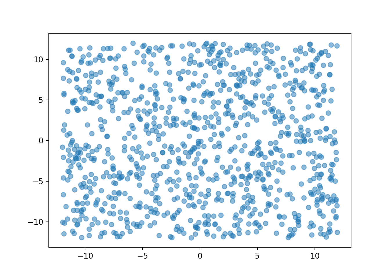
10.11 Solution to Exercise 3.11
P = Uniform(1, 4) ** 2

X = RV(P, sum)
Y = RV(P, max)

(RV(P) & X & Y).sim(10)| Index | Result |
|---|---|
| 0 | ((1.860895916307121, 1.9289785804701047), 3.7898744967772258, 1.9289785804701047) |
| 1 | ((3.2504651519330983, 1.531622468836602), 4.7820876207697, 3.2504651519330983) |
| 2 | ((3.914065727984431, 1.4435643518088548), 5.357630079793285, 3.914065727984431) |
| 3 | ((3.770243618491405, 3.092897348281372), 6.863140966772777, 3.770243618491405) |
| 4 | ((2.500488701813131, 3.3032774445223234), 5.803766146335454, 3.3032774445223234) |
| 5 | ((3.1157165653791994, 1.7764737705456886), 4.892190335924888, 3.1157165653791994) |
| 6 | ((3.8370747868685764, 2.359990750339249), 6.197065537207825, 3.8370747868685764) |
| 7 | ((1.0161349508256863, 2.666187449292412), 3.6823224001180983, 2.666187449292412) |
| 8 | ((1.5285975932710545, 1.368095094318643), 2.8966926875896974, 1.5285975932710545) |
| ... | ... |
| 9 | ((3.912936485595191, 1.9351231116431848), 5.848059597238375, 3.912936485595191) |
plt.figure()
(X & Y).sim(1000).plot()
plt.show()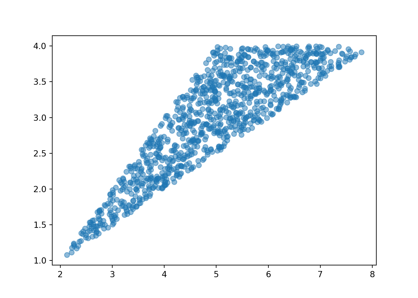
10.12 Solution to Exercise 3.12
Part 1
See previous solutions which discuss how to simulate \((X, Y)\) pairs.
Simulate many \((X, Y)\) pairs, say 10000.
- To approximate \(\textrm{P}(X = 2)\): Divide the number of repetitions with \(X = 2\) by the total number of repetitions
- To approximate \(\textrm{P}(Y = 1)\): Divide the number of repetitions with \(Y = 1\) by the total number of repetitions
- To approximate \(\textrm{P}(X = 2, Y = 1)\): Divide the number of repetitions with \(X = 2\) and \(Y=1\) by the total number of repetitions
Part 2
P = BoxModel([1, 2, 3], size = 3)

def count_distinct(u):
    return len(set(u))

X = RV(P, count_distinct)

Y = RV(P, count_eq(1))

x_and_y = (X & Y).sim(10000)

x = x_and_y[0]

y = x_and_y[1]x.count_eq(2) / x.count()0.6648y.count_eq(1) / x.count()0.4463((x == 2) * (y == 1)).sum() / x.count()0.2249Part 3
x.tabulate(normalize = True)| Value | Relative Frequency |
|---|---|
| 1 | 0.1138 |
| 2 | 0.6648 |
| 3 | 0.2214 |
| Total | 1.0 |
plt.figure()
x.plot()
plt.show()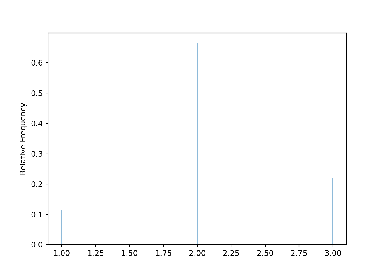
y.tabulate(normalize = True)| Value | Relative Frequency |
|---|---|
| 0 | 0.2948 |
| 1 | 0.4463 |
| 2 | 0.2218 |
| 3 | 0.0371 |
| Total | 1.0 |
plt.figure()
y.plot()
plt.show()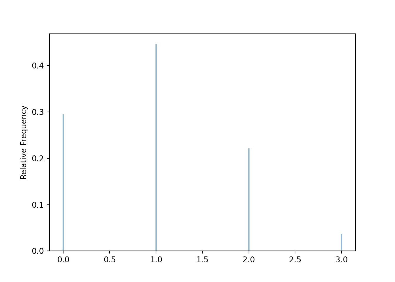
x_and_y.tabulate(normalize = True)| Value | Relative Frequency |
|---|---|
| (1, 0) | 0.0767 |
| (1, 3) | 0.0371 |
| (2, 0) | 0.2181 |
| (2, 1) | 0.2249 |
| (2, 2) | 0.2218 |
| (3, 1) | 0.2214 |
| Total | 1.0 |
plt.figure()
x_and_y.plot('tile')
plt.show()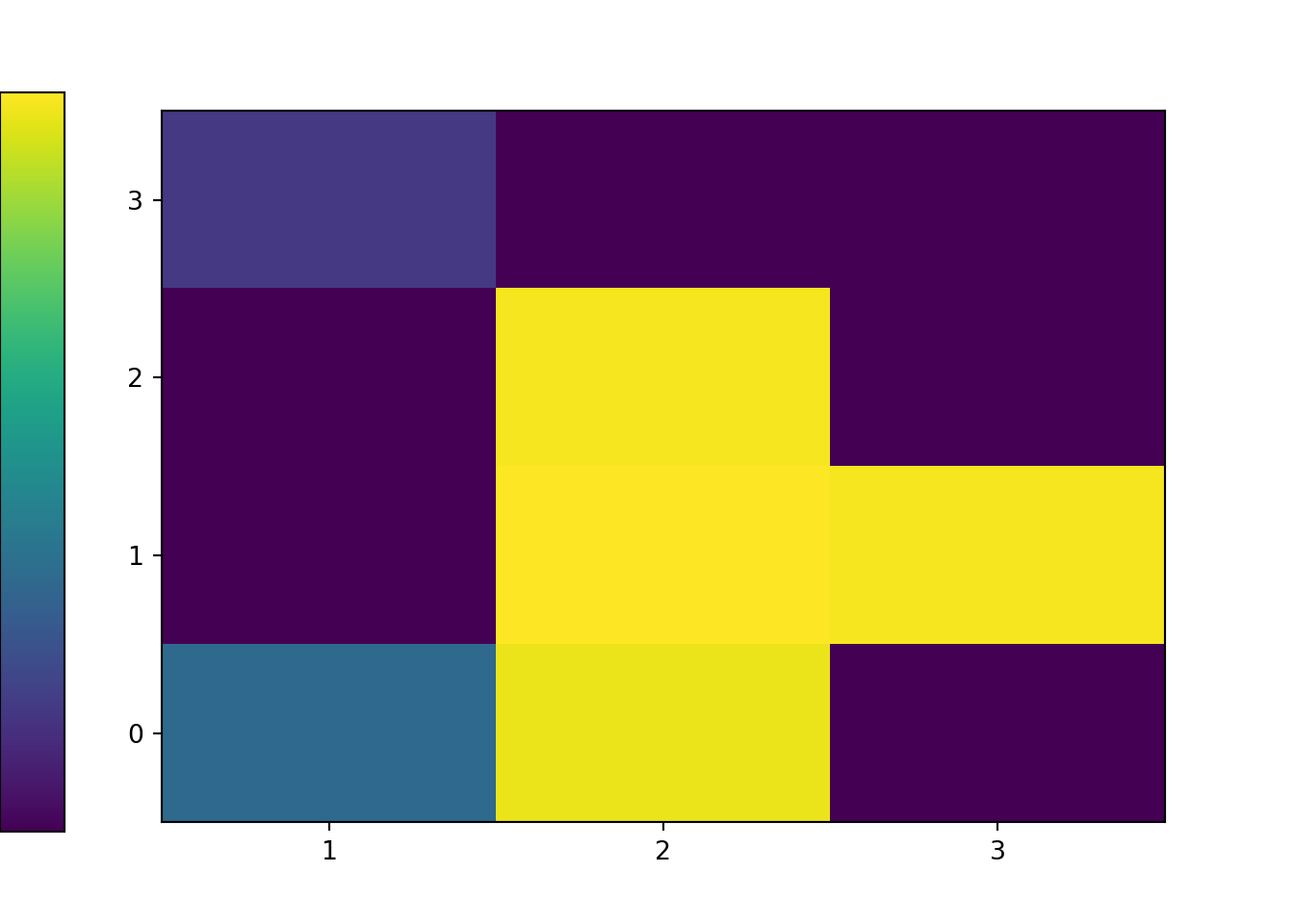
10.13 Solution to Exercise 3.13
Part 1
See previous solutions which discuss how to simulate \((X, Y)\) pairs.
Simulate many \((X, Y)\) pairs, say 10000.
- To approximate \(\textrm{P}(X = 2)\): Divide the number of repetitions with \(X = 2\) by the total number of repetitions
- To approximate \(\textrm{P}(Y = 1)\): Divide the number of repetitions with \(Y = 1\) by the total number of repetitions
- To approximate \(\textrm{P}(X = 2, Y = 1)\): Divide the number of repetitions with \(X = 2\) and \(Y=1\) by the total number of repetitions
Part 2
P = BoxModel([1, 2, 3], size = 3, probs = [0.1, 0.3, 0.6])

def count_distinct(u):
    return len(set(u))

X = RV(P, count_distinct)

Y = RV(P, count_eq(1))

x_and_y = (X & Y).sim(10000)

x = x_and_y[0]

y = x_and_y[1]x.count_eq(2) / x.count()0.6426y.count_eq(1) / x.count()0.2461((x == 2) * (y == 1)).sum() / x.count()0.1366Part 3
x.tabulate(normalize = True)| Value | Relative Frequency |
|---|---|
| 1 | 0.2479 |
| 2 | 0.6426 |
| 3 | 0.1095 |
| Total | 1.0 |
plt.figure()
x.plot()
plt.show()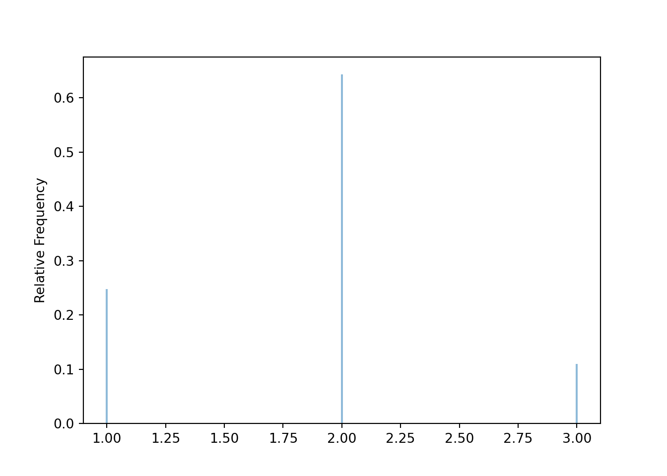
y.tabulate(normalize = True)| Value | Relative Frequency |
|---|---|
| 0 | 0.725 |
| 1 | 0.2461 |
| 2 | 0.028 |
| 3 | 0.0009 |
| Total | 1.0 |
plt.figure()
y.plot()
plt.show()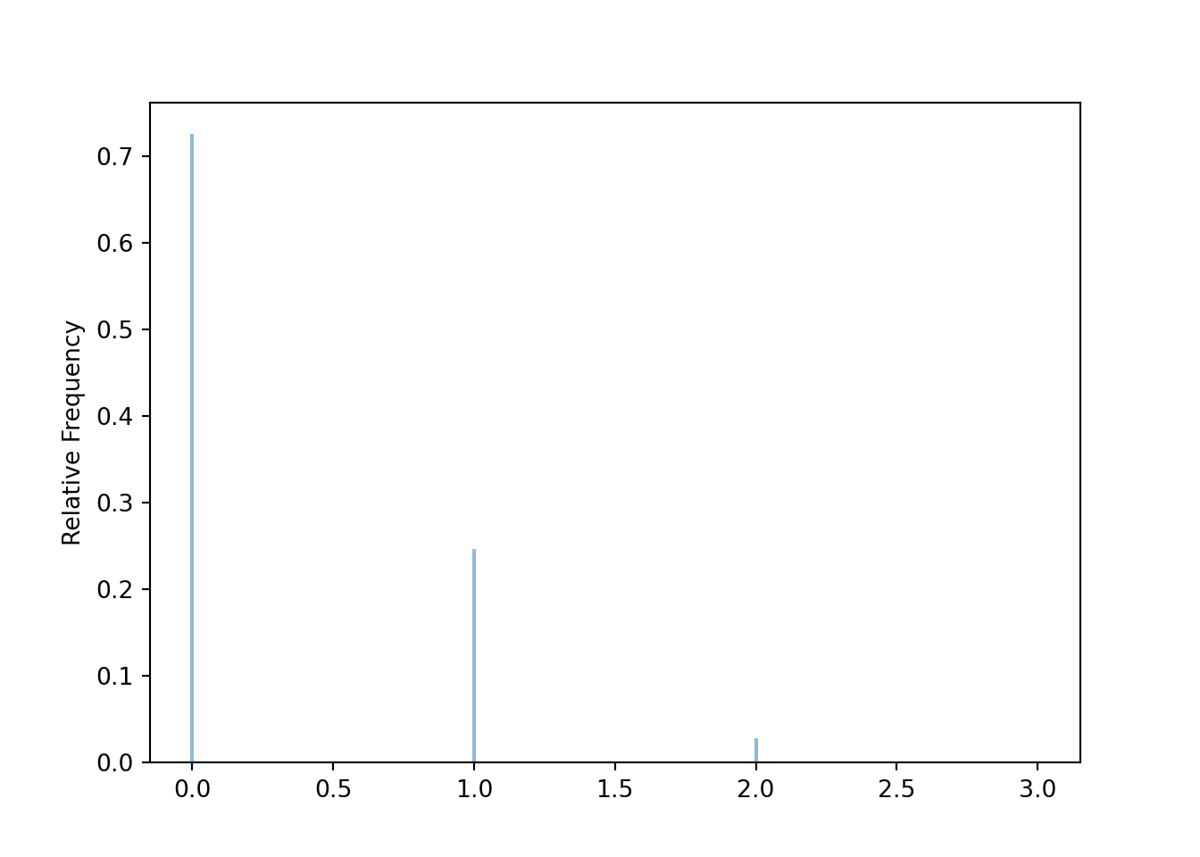
x_and_y.tabulate(normalize = True)| Value | Relative Frequency |
|---|---|
| (1, 0) | 0.247 |
| (1, 3) | 0.0009 |
| (2, 0) | 0.478 |
| (2, 1) | 0.1366 |
| (2, 2) | 0.028 |
| (3, 1) | 0.1095 |
| Total | 1.0 |
plt.figure()
x_and_y.plot('tile')
plt.show()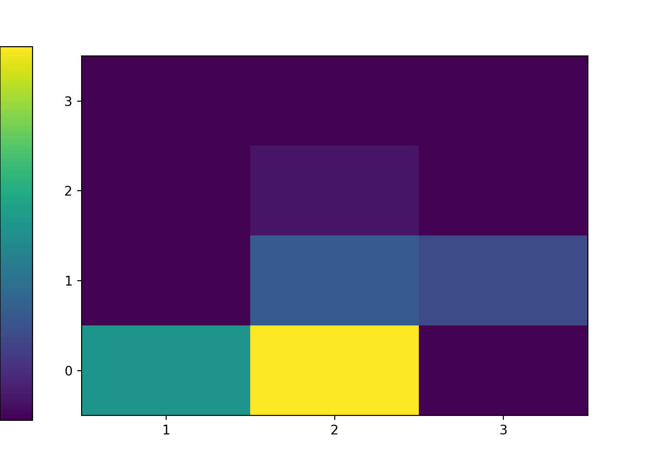
10.14 Solution to Exercise 3.14
Part 1
See previous solutions for description of how to simulate values of \(X\).
Simulate many values of \(X\) and summarize the simulate values and their relative frequencies to approximate the distribution of \(X\).
To approximate \(\textrm{P}(X > 3)\): divide the number of repetitions with \(X>3\) by the total number of repetitions.
Part 2
p_success = 0.4

# define a function that takes as an input a sequence of 0s and 1s (omega)
# and returns when the first 1 occurs
def count_until_first_success(omega):
    for i, w in enumerate(omega):
        if w == 1:
            return i + 1 # the +1 is for zero-based indexing

# Either of the following probability spaces works
# P = Bernoulli(p_success) ** inf
P = BoxModel([1, 0], probs = [p_success, 1 - p_success], size = inf)

X = RV(P, count_until_first_success)

x = X.sim(10000)

x| Index | Result |
|---|---|
| 0 | 1 |
| 1 | 1 |
| 2 | 1 |
| 3 | 1 |
| 4 | 5 |
| 5 | 1 |
| 6 | 1 |
| 7 | 4 |
| 8 | 1 |
| ... | ... |
| 9999 | 2 |
x.tabulate(normalize = True)| Value | Relative Frequency |
|---|---|
| 1 | 0.3919 |
| 2 | 0.2451 |
| 3 | 0.1402 |
| 4 | 0.088 |
| 5 | 0.0516 |
| 6 | 0.0328 |
| 7 | 0.0201 |
| 8 | 0.0125 |
| 9 | 0.0069 |
| 10 | 0.0043 |
| 11 | 0.0034 |
| 12 | 0.0011 |
| 13 | 0.0009 |
| 14 | 0.0004 |
| 15 | 0.0002 |
| 16 | 0.0003 |
| 17 | 0.0002 |
| 20 | 0.0001 |
| Total | 1.0 |
plt.figure()
x.plot()
plt.show()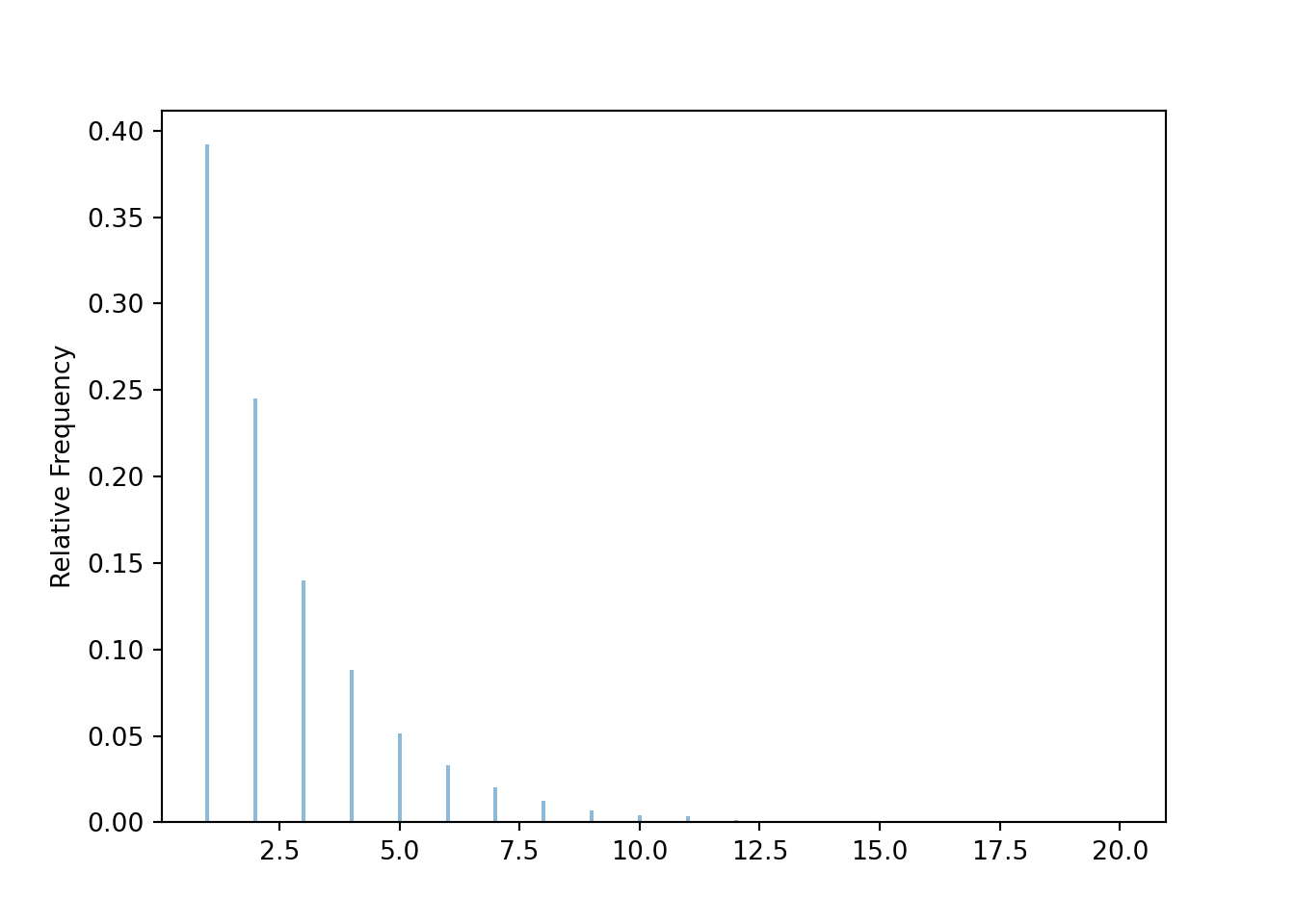
x.count_gt(3) / x.count()0.222810.15 Solution to Exercise 3.15
Part 1
See previous solutions for how to simulate \((X, Y)\) pairs.
Simulate many \((X, Y)\) pairs, say 10000. To approximate:
- \(\textrm{P}(X < 3.5)\): divide number of repetitions with \(X<3.5\) by the total number of repetitions
- \(\textrm{P}(Y > 2.7)\): divide number of repetitions with \(Y>2.7\) by the total number of repetitions
- \(\textrm{P}(X < 3.5, Y > 2.7)\): divide number of repetitions with \(X<3.5\) and \(Y>2.7\) by the total number of repetitions
Part 2
We usually summarize simulated values of continuous random variables with histogram.
P = Uniform(1, 4) ** 2

X = RV(P, sum)
Y = RV(P, max)

x_and_y = (X & Y).sim(10000)

x = x_and_y[0]

y = x_and_y[1]
plt.figure()
x.plot()
plt.show()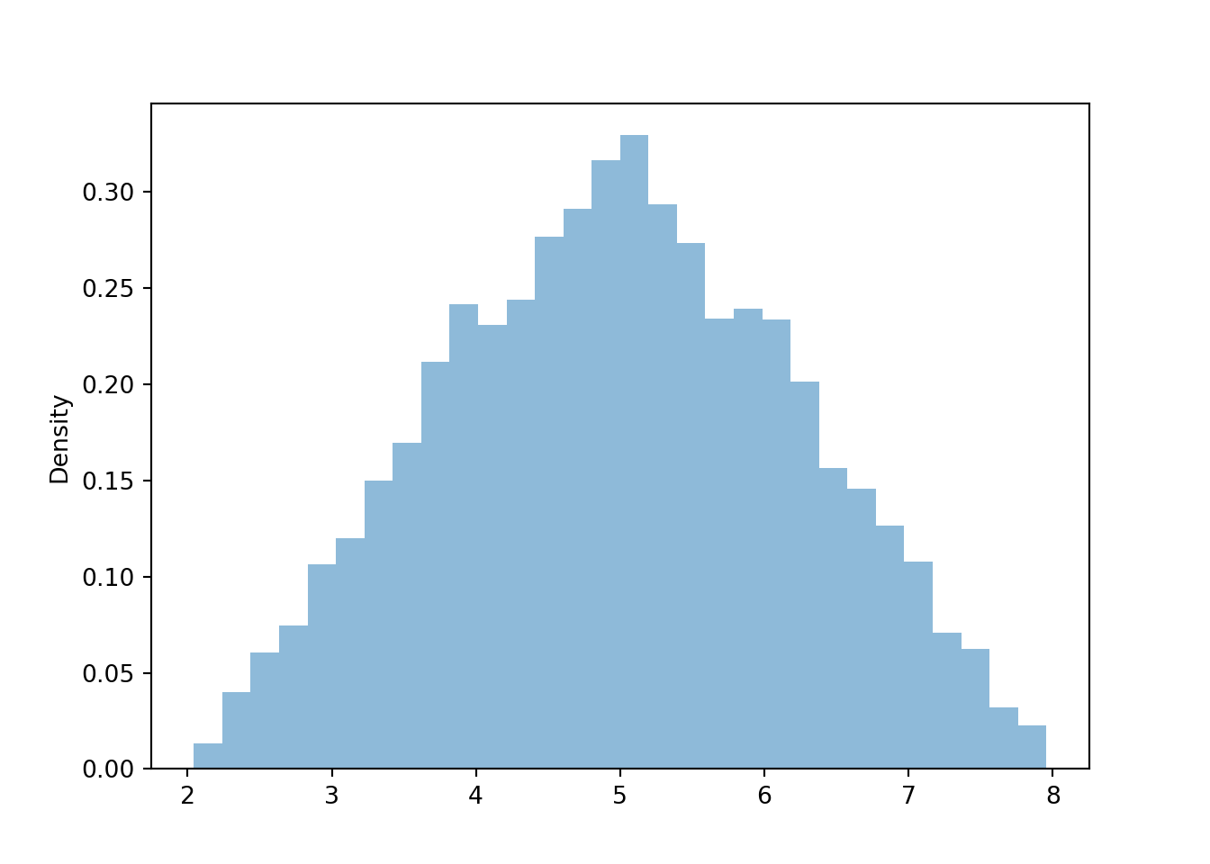
plt.figure()
y.plot()
plt.show()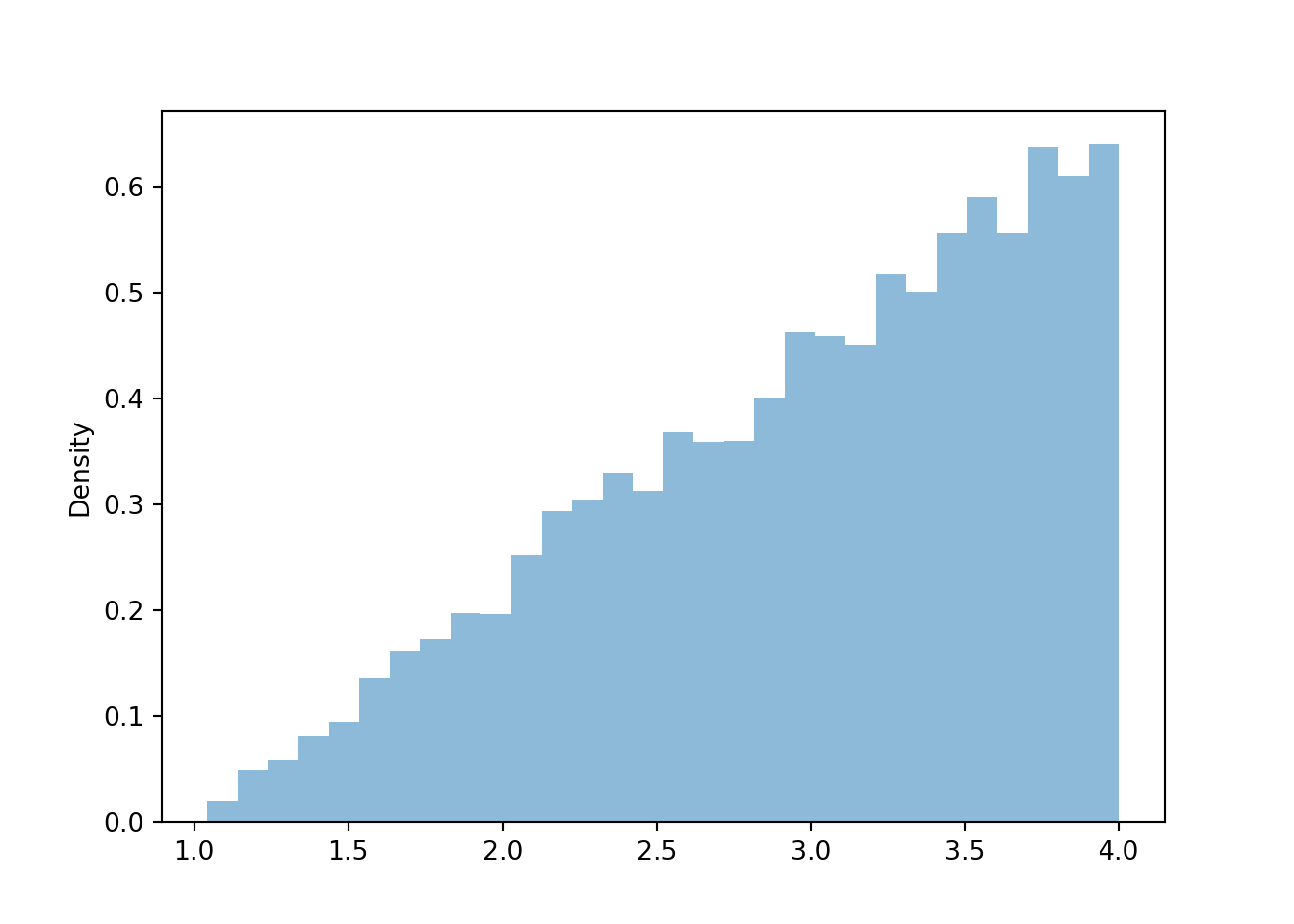
plt.figure()
x_and_y.plot()
plt.show()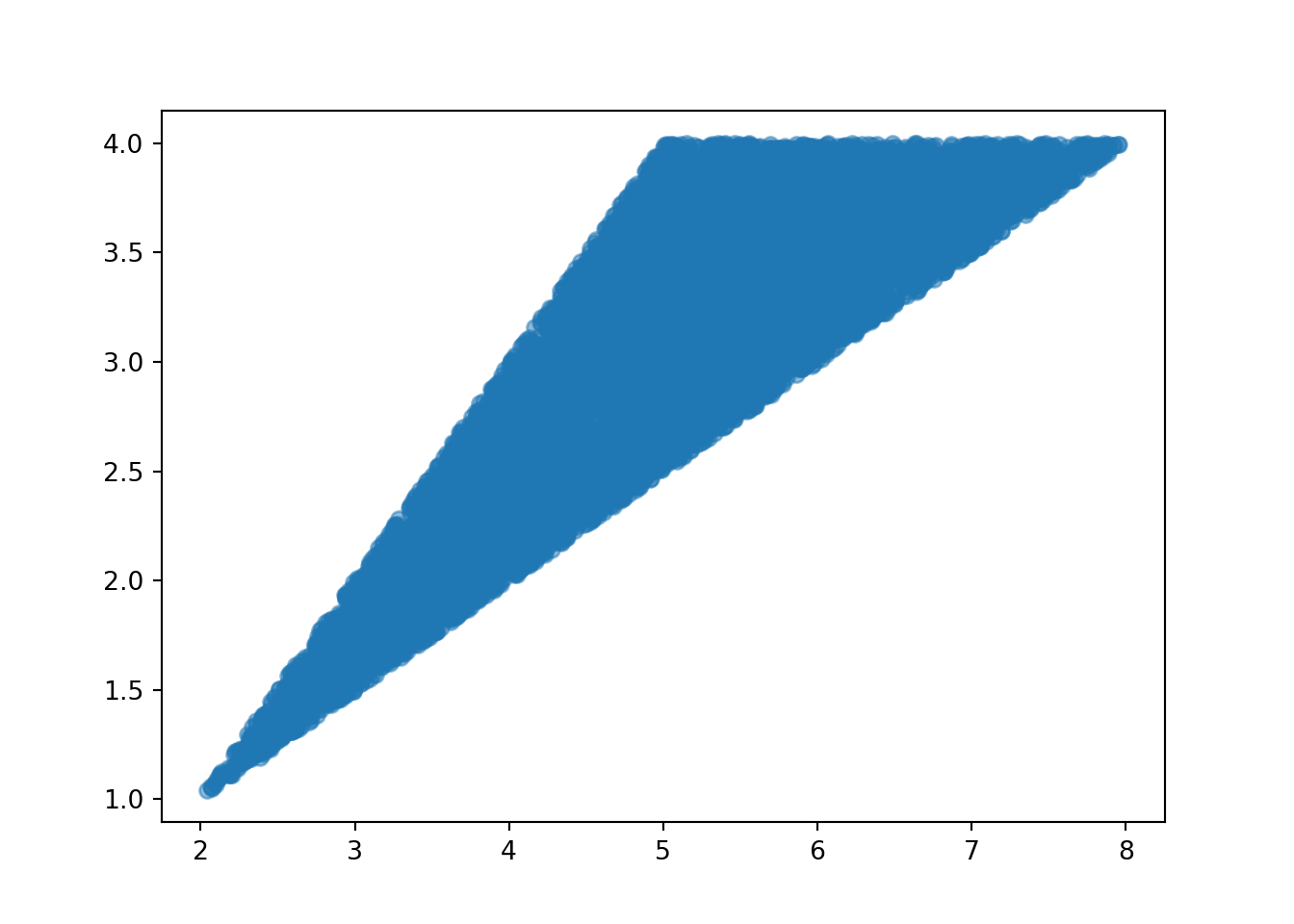
plt.figure()
x_and_y.plot('hist')
plt.show()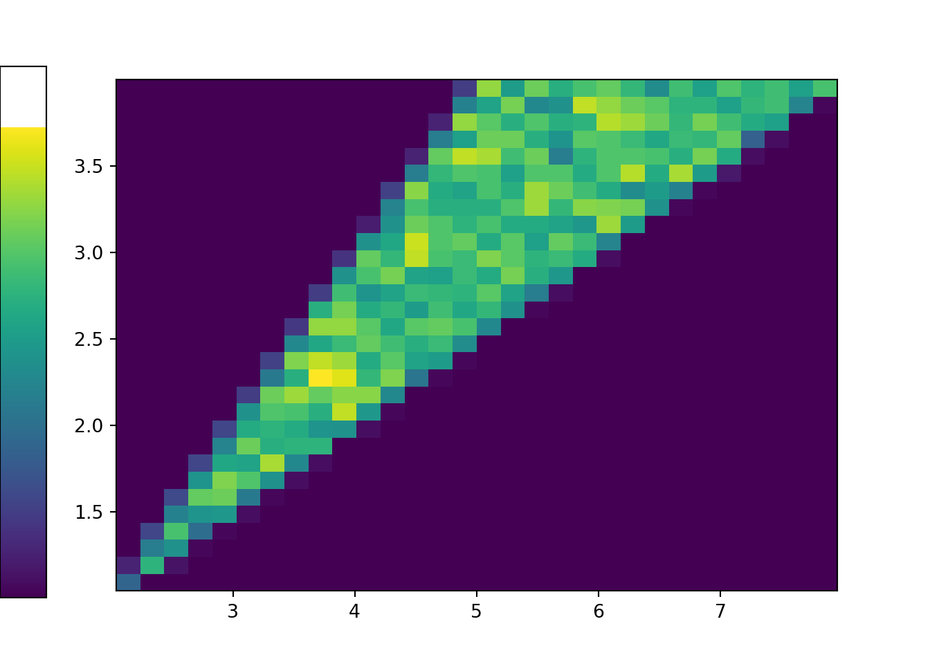
10.16 Solution to Exercise 3.16
Simulate 10000 repetitions and find the relative frequency of repetitions on which at least 2 people share a birthday. The margin of error is \(1/\sqrt{10000} = 0.01\)
n = 30

P = BoxModel(list(range(365)), size = n)

def count_distinct(u):
  return len(set(u))

X = RV(P, count_distinct)

B = (X < n)

p_hat = B.sim(10000).count_eq(True) / 10000

p_hat0.7124We estimate (with 95% confidence) that the probability that at least two people in a group of 30 share the same birthday is 0.712 with a margin of error of 0.01. In other words, we estimate (with 95% confidence) that the probability that at least two people in a group of 30 share the same birthday is between 0.7 and 0.72.
10.17 Solution to Exercise 3.17
The margin of error for any single probability would be \(1/\sqrt{10000} = 0.01\), but since we are estimating many probabilities simultaneously we would use a margin of error of \(2\times 0.01\). For example, if the simulated relative frequency of \(X = 2\) is 0.662, then we approximate \(\textrm{P}(X = 2)\) to be 0.662 with a margin of error of 0.02; in other words, we estimate that \(\textrm{P}(X = 2)\) is between 0.642 and 0.682.
10.18 Solution to Exercise 3.18
- \(X\) takes the value 210 with probability 1/5 and 35 with probability 4/5.
- \(\text{E}(X) = 210(1/5) + 35(4/5)=70\) is the average number of students per class from the instructors’ perspective. If we randomly select an instructor, record the number of students in the instructor’s class, and repeat, the long run average number of students will be 70.
- \(\text{P}(X = \text{E}(X)) = \text{P}(X = 70) = 0\). No instructor has a class whose size is equal to the average class size (from the instructor’s perspective).
- \(Y\) takes the value 210 with probability 210/350 and 35 with probability 140/350.
- \(\text{E}(Y) = 210(210/350) + 35(140/350)=140\) is the average number of students per class from the students’ perspective. If we randomly select a student, record the number of students in the selected student’s class, and repeat, the long run average number of students will be 140.
- \(\text{P}(Y = \text{E}(Y)) = \text{P}(Y = 140) = 0\). No student is in a class whose size is equal to the average class size (from the students’ perspective).
- Colleges usually report average class size from the instructor/class perspective, which in this case would be 70 students. From the students’ perspective, the average class size is not even close to 70! In fact, it’s twice that size. Some students (140 of them, which is 40% of the total of 350 students) have the benefit of a small class size of 35. But most students (210 of them, which is 60% of the students) are stuck in a large class of 210 students. In other words, most students would be pretty seriously misled if they chose this college based on the advertised average class size of 35 students per class. From the students’ perspective, it seems that 140 is the more relevant average to report. However, neither average really adequately represents what is happening here: there is wide variability in class sizes between large and small.
10.19 Solution to Exercise 3.19
See previous for solutions for how to simulate \((X, Y)\) pairs
Part 1
Simulate many \((X, Y)\) pairs, say 10000
- To approximate \(\textrm{E}(X)\): average the simulated \(X\) values (sum the 10000 simulated \(X\) values and divide by 10000)
- To approximate \(\textrm{E}(Y)\): average the simulated \(Y\) values (sum the 10000 simulated \(Y\) values and divide by 10000)
- To approximate \(\textrm{E}(X^2)\): average the simulated \(X^2\) values (square each simulated \(X\) value then sum the 10000 \(X^2\) values and divide by 10000)
- To approximate \(\textrm{E}(XY)\): average the simulated \(XY\) values (for each \((X, Y)\) pair compute the product \(XY\) then sum the 10000 \(XY\) values and divide by 10000)
Part 2
P = BoxModel([1, 2, 3], size = 3)

def count_distinct(u):
    return len(set(u))

X = RV(P, count_distinct)

Y = RV(P, count_eq(1))

x_and_y = (X & Y).sim(10000)

x = x_and_y[0]

y = x_and_y[1]x.mean()2.1141y.mean()1.0045(x ** 2).mean()4.7895(x * y).mean()2.121610.20 Solution to Exercise 3.20
See previous for solutions for how to simulate \((X, Y)\) pairs
Part 1
Simulate many \((X, Y)\) pairs, say 10000
- To approximate \(\textrm{E}(X)\): average the simulated \(X\) values (sum the 10000 simulated \(X\) values and divide by 10000)
- To approximate \(\textrm{E}(Y)\): average the simulated \(Y\) values (sum the 10000 simulated \(Y\) values and divide by 10000)
- To approximate \(\textrm{E}(X^2)\): average the simulated \(X^2\) values (square each simulated \(X\) value then sum the 10000 \(X^2\) values and divide by 10000)
- To approximate \(\textrm{E}(XY)\): average the simulated \(XY\) values (for each \((X, Y)\) pair compute the product \(XY\) then sum the 10000 \(XY\) values and divide by 10000)
Part 2
P = Uniform(1, 4) ** 2

X = RV(P, sum)

Y = RV(P, max)

x_and_y = (X & Y).sim(10000)

x = x_and_y[0]

y = x_and_y[1]x.mean()5.022143026247546y.mean()3.009975330790258(x ** 2).mean()26.718306370950874(x * y).mean()15.85697585837203110.21 Solution to Exercise 3.21
See previous parts for how to simulate \(X\) values.
Part 1
To approximate \(\textrm{Var}(X)\):
- Simulate many \(X\) values and compute the average of the simulated values
- Square each simulated \(X\) value and compute the average of the squared values
- Subrtract the square of the average from part a) from the average of the squares in part b).
Part 2
P = BoxModel([1, 2, 3], size = 3)

def count_distinct(u):
    return len(set(u))

X = RV(P, count_distinct)

x = X.sim(10000)
(x ** 2).mean() - (x.mean()) ** 20.3219900399999993x.var()0.32199004000000003x.sd()0.567441662199736710.22 Solution to Exercise 3.22
Part 1
P = Uniform(1, 4) ** 2

X = RV(P, sum)

Y = RV(P, max)

x_and_y = (X & Y).sim(10000)

x = x_and_y[0]

y = x_and_y[1]
x.plot()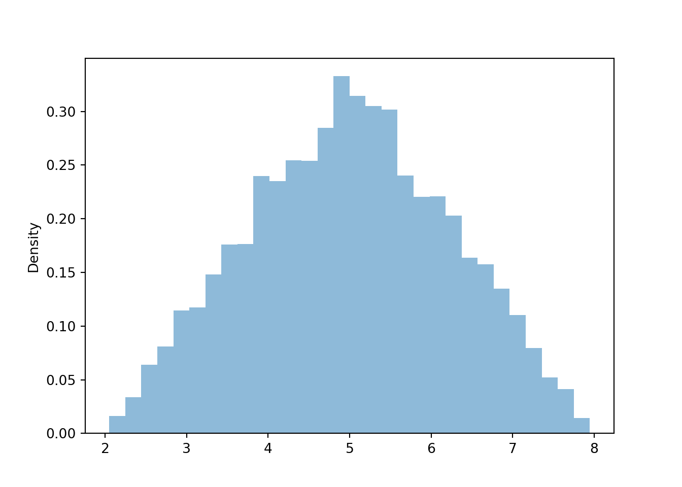
y.plot()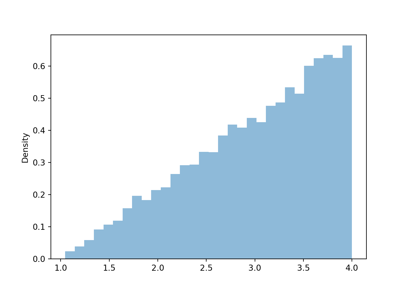
Part 2
\(X\) will have larger standard deviation than \(Y\). The values of \(X\) range from 2 to 8 while the values of \(Y\) only range from 1 to 4. Also, the values of \(Y\) tend to be closer to their mean (around 3.0) than the values of \(X\) are to their mean (around 5).
The values of \(X\) can be anywhere from 0 to 3 units away from the mean of 5, but more values are closer than farther; we might estimate the SD to be less than 1.5. (Remember, the squaring then averaging then taking the square root makes it hard to guess the actual number)
We would estimate the SD of \(Y\) to be less that of \(X\), and maybe a little less than 1, since a large percentage of values are between 2 and 4 (hence less than 1 unit away from the mean).
Part 3
To approximate \(\textrm{Var}(X)\):
- Simulate many \(X\) values and compute the average of the simulated values
- Square each simulated \(X\) value and compute the average of the squared values
- Subrtract the square of the average from part a) from the average of the squares in part b).
Take the square of the variance to approximate the standard deviation.
Similarly for \(Y\).
Part 4
x.var(), x.sd()(1.5047072917149114, 1.2266651098465755)y.var(), y.sd()(0.49861141691726896, 0.7061242220156939)10.23 Solution to Exercise 10.1
Exercise 10.1
- Explain how you could, in principle, conduct a simulation by hand and use the results to approximate \(\textrm{Cov}(X, Y)\).
- Write Symbulate code to conduct a simulation and approximate the covariance and correlation.
- Compute \(\textrm{Cov}(X, Y)\) and \(\textrm{Corr}(X, Y)\).
- Are \(X\) and \(Y\) independent? Explain your reasoning.
- See previous solutions for how to simulate \((X, Y)\) pairs.
- Simulate many \((X, Y)\) pairs
- Compute the average of the simulated \(X\) values (i.e., sum the simulated values of \(X\) and divide by the number of simulated values) to approximate \(\textrm{E}(X)\)
- Compute the average of the simulated \(Y\) values (i.e., sum the simulated values of \(Y\) and divide by the number of simulated values) to approximate \(\textrm{E}(Y)\)
- Find the product \(XY\) for each pair, and compute the average value of the products (i.e., sum the simulated values of \(XY\) and divide by the number of simulated pairs) to approximate \(\textrm{E}(XY)\)
- Subract the approximations \(\textrm{E}(XY) - \textrm{E}(X)\textrm{E}(Y)\) to approximate \(\textrm{Cov}(X, Y)\)
- See code below
- In Exercise 2.16 we found the joint distribution of \(X\) and \(Y\) in a previous problem, and also computed \(\textrm{E}(X) = 57/27 = 2.111\) and \(\textrm{E}(Y)=1\). In computing \(\textrm{E}(XY)\) many of the terms are 0, either because one of \(Y\) is 0 or because the probability of the pair is 0 \[ \textrm{E}(XY) = (1)(3)(1/27) + (2)(1)(6/27) + (2)(2)(6/27) + (3)(1)(6/27) + 0 = 57/27 = 2.111 \] So \(\textrm{Cov}(X, Y) = \textrm{E}(XY) - \textrm{E}(X)\textrm{E}(Y) = 57/27 - (57/27)(1) = 0\). Therefore \(\textrm{Corr}(X, Y) = 0\) and \(X\) and \(Y\) are uncorrelated.
- Even though the covariance is 0, \(X\) and \(Y\) are not independent. For example \(\textrm{P}(X = 1) = 3/27\) but \(\textrm{P}(X = 1|Y=1) = 0\). Knowing the value of \(Y\) changes the distribution of \(X\), and vice versa.
10.24 Solution to Exercise 3.24
\(X\) takes values 0, 1, 2, 3. One outcome corresponds to each of \(X=0\) (LLL) and \(X=3\) (WWW), and 3 outcomes correpond to each of \(X=1\) (WLL, LWL, LLW) and \(X=2\) (WWL, WLW, LWW), but the outcomes are not equally likely.
\(x\) Outcomes \(\textrm{P}(X = X)\) 0 LLL \((1)(18/38)^0(20/38)^3=0.146\) 1 WLL, LWL, LLW \((3)(18/38)^1(20/38)^2=0.394\) 2 WWL, WLW, LWW \((3)(18/38)^2(20/38)^1=0.354\) 3 WWW \((1)(18/38)^3(20/38)^0=0.106\) \(\text{E}(X)=0(0.146)+1(0.394)+2(0.354)+3(0.106)= 1.42\).
\(\text{E}(X^2)=0^2(0.146)+1^2(0.394)+2^2(0.354)+3^2(0.106)= 2.76\), so \(\textrm{Var}(X)=0.75\).
In the first 3 bets Yolanda wins the same number of games as Xavier, and Yolanda only plays two more games. So \(Y\) can’t be more than \(X+2\), and \(Y\) can’t be less than \(X\).
To have \(X = 2\) and \(Y=3\) we need to have exactly two wins in the first 3 bets (where both play) and exactly 1 win in the last 2 bets (Yolanda only). \[ \text{P}(X = 2, Y = 3) = \left((3)(18/38)^2(20/38)^1\right)\left((2)(18/38)^1(20/38)^1\right) = 0.177 \]
\(X\) and \(Y\) are not independent. For example, \(\textrm{P}(X = 1, Y = 0)=0\) which is not \(\textrm{P}(X=1)\textrm{P}(Y=0)\).
\(\textrm{P}(X + Y = 4) = 0.0883+0.0981 = 0.1864\).
Sum the appropriate values from the joint distribution table.
\(z\) \(\textrm{P}(X+Y = z)\) 0 0.0404 1 0.0727 2 0.1417 3 0.1963 4 0.1864 5 0.1766 6 0.1089 7 0.0530 8 0.0238 Use the table from the previous part to compute \(\text{E}(X+Y) = 3.79\).
\(\textrm{E}(XY) = 4.11\) so \(\textrm{Cov}(X, Y) = 4.11 - (1.42)(2.37) = 0.75\). There is a positive association; if \(X\) is large that means Xavier won a lot of games so Yolanda tends to win more games too.
\(\textrm{Corr}(X, Y) = 0.75/\sqrt{(0.75)(1.25)} = 0.77\).
10.25 Solution to Exercise 3.25
Approximate the conditional distribution of \(Y\) given \(X=1\):
- Simulate \((X, Y)\) pair
- If \(X\neq1\) discard the repetition, otherwise keep
- Repeat until 10000 repetitions with \(X=1\) are obtained
- Summarize the simulated values of \(Y\) from these repetitions to approximate the conditional distribution of \(Y\) given \(X = 1\)
- To approximate \(\textrm{P}(Y = 0 | X=1)\) count the number of repetitions with \(Y=0\) and divide by 10000 (remember, all of the repetitions have \(X = 1\))
Approximate the conditional distribution of \(X\) given \(Y=0\) similarly, with a different simulation of 10000 \((X, Y)\) pairs that satisfy \(Y=0\).
P = BoxModel([1, 2, 3], size = 3)

def count_distinct(u):
    return len(set(u))

X = RV(P, count_distinct)

Y = RV(P, count_eq(1))
y_given_Xeq1 = ( Y | (X == 1) ).sim(10000)y_given_Xeq1.tabulate()| Value | Frequency |
|---|---|
| 0 | 6686 |
| 3 | 3314 |
| Total | 10000 |
y_given_Xeq1.tabulate(normalize=True)| Value | Relative Frequency |
|---|---|
| 0 | 0.6686 |
| 3 | 0.3314 |
| Total | 1.0 |
plt.figure()
y_given_Xeq1.plot()
plt.show()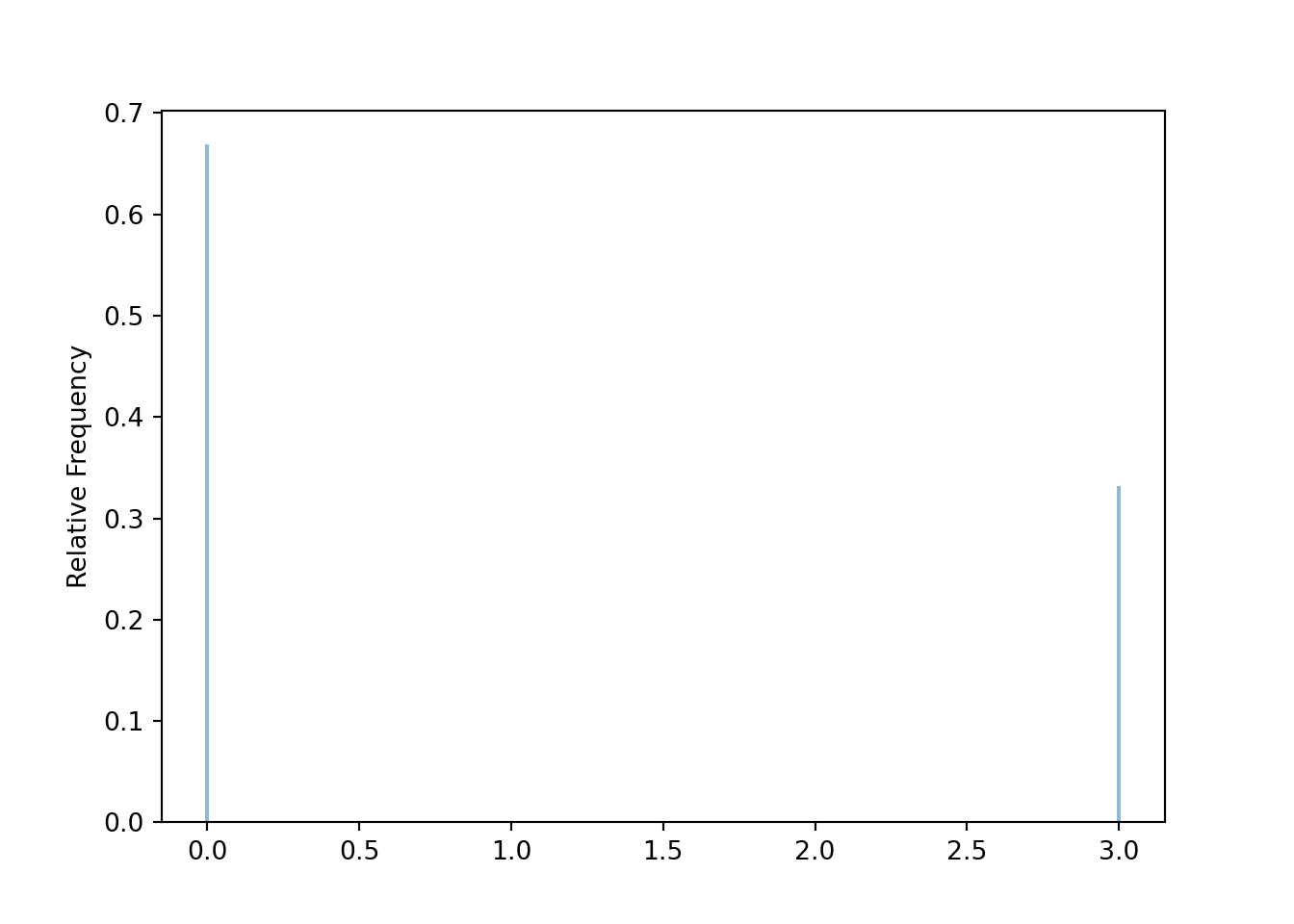
x_given_Yeq0 = ( X | (Y == 0) ).sim(10000)x_given_Yeq0.tabulate()| Value | Frequency |
|---|---|
| 1 | 2507 |
| 2 | 7493 |
| Total | 10000 |
x_given_Yeq0.tabulate(normalize=True)| Value | Relative Frequency |
|---|---|
| 1 | 0.2507 |
| 2 | 0.7493 |
| Total | 1.0 |
plt.figure()
x_given_Yeq0.plot()
plt.show()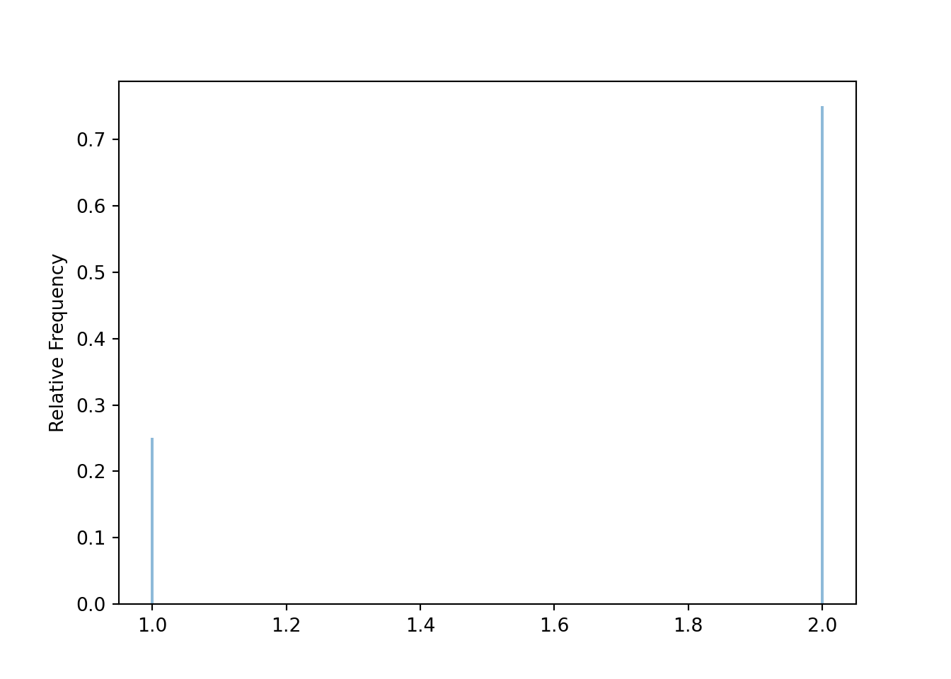
10.26 Solution to Exercise 3.26
In the code below
Uniform(0, 12) ** 2corresponds to the two spinsBoxModel([-1, 1], size = 2)corresponds to the two coin flipsUniform(0, 12) ** 2 * BoxModel([-1, 1], size = 2)simulates a pair which we unpack and define asRVsU, F, butUis itself a pair and so isF.U[0]is the first spin andF[0]is the first flip.
U, F = RV(Uniform(0, 12) ** 2 * BoxModel([-1, 1], size = 2))

X = U[0] * F[0]

Y = U[1] * F[1]

R = sqrt(X ** 2 + Y ** 2)

( (U & F & X & Y & R) | (R < 12) ).sim(10)| Index | Result |
|---|---|
| 0 | ((2.518045958638199, 7.536195215801989), (-1, 1), -2.518045958638199, 7.536195215801989, 7.945740606... |
| 1 | ((2.20886638224083, 6.99798522454787), (1, -1), 2.20886638224083, -6.99798522454787, 7.3383164211952... |
| 2 | ((9.453478205546002, 5.162916700939377), (-1, 1), -9.453478205546002, 5.162916700939377, 10.77144182... |
| 3 | ((9.688587076583554, 6.370902891519927), (1, 1), 9.688587076583554, 6.370902891519927, 11.5955648070... |
| 4 | ((10.808786054243297, 1.910932274344808), (1, 1), 10.808786054243297, 1.910932274344808, 10.97640734... |
| 5 | ((4.796921443499318, 2.814938303273778), (-1, 1), -4.796921443499318, 2.814938303273778, 5.561864164... |
| 6 | ((1.468640635764245, 1.054798499553189), (1, 1), 1.468640635764245, 1.054798499553189, 1.80817731201... |
| 7 | ((10.066097257353276, 3.7115465380670183), (-1, 1), -10.066097257353276, 3.7115465380670183, 10.7285... |
| 8 | ((0.977490913076815, 10.680824141422573), (1, 1), 0.977490913076815, 10.680824141422573, 10.72546002... |
| ... | ... |
| 9 | ((8.143505049488244, 0.24976089583871275), (-1, 1), -8.143505049488244, 0.24976089583871275, 8.14733... |
plt.figure()
( (X & Y) | (R < 12) ).sim(1000).plot()
plt.show()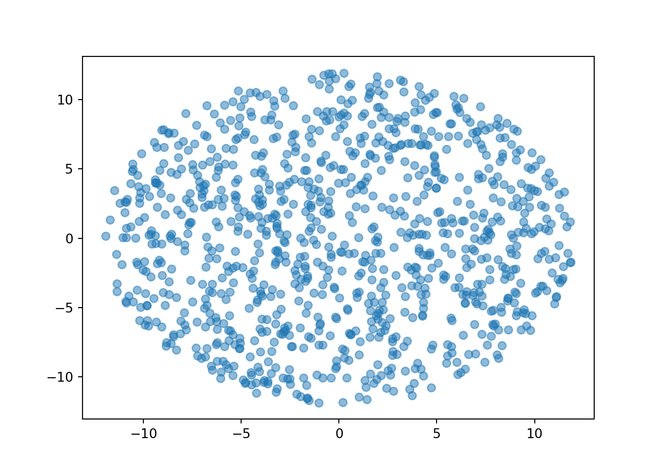
r = ( R | (R < 12) ).sim(10000)

plt.figure()
r.plot()
plt.show()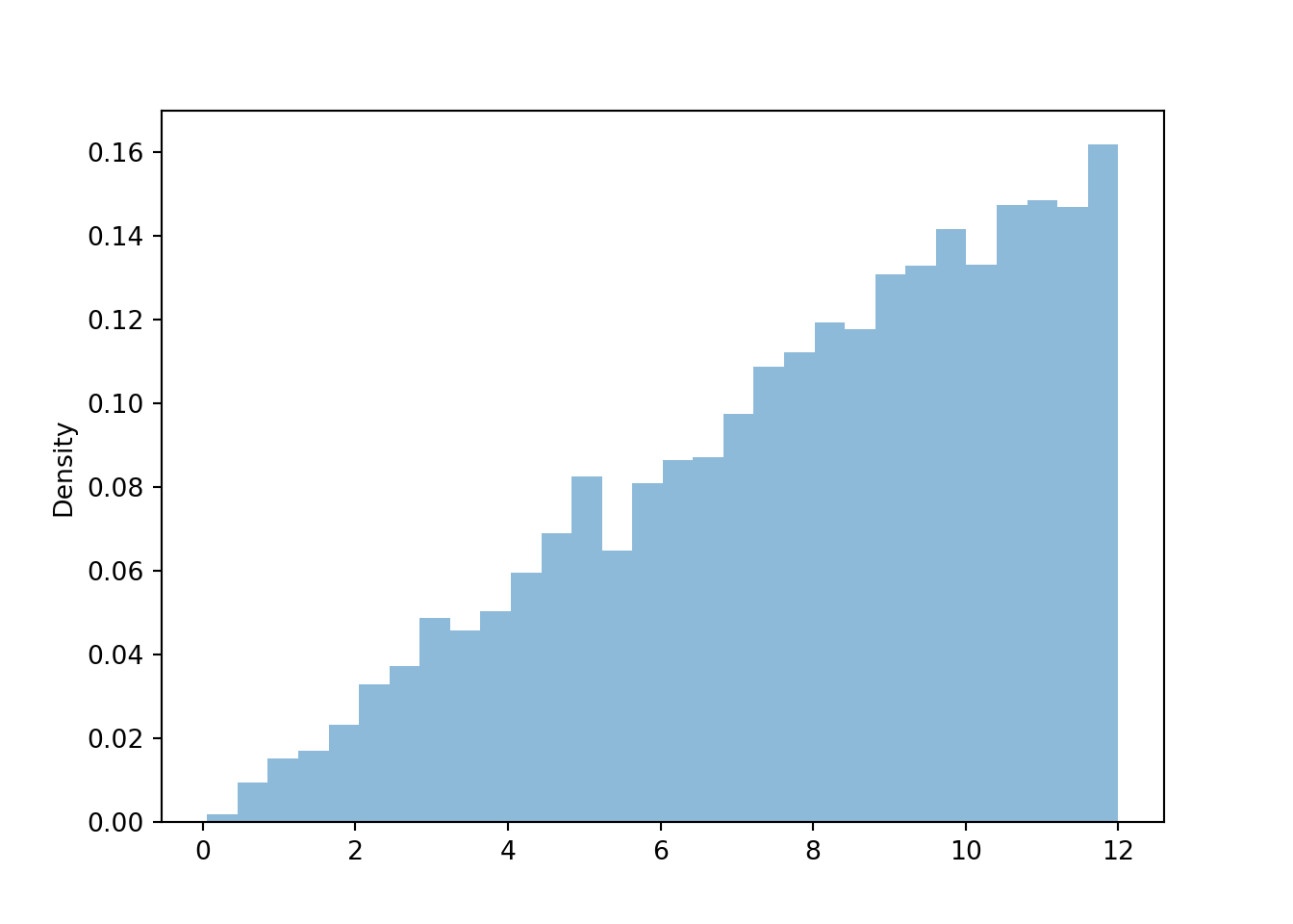
r.count()10000r.count_lt(1) / r.count()0.0063r.count_gt(11) / r.count()0.1519r.mean()7.971670084479064r.sd()2.81027432192058610.27 Solution to Exercise 3.27
We condition on \(X\) being “close to” 3.5, say within 0.1 of 3.5
P = Uniform(1, 4) ** 2

X = RV(P, sum)

Y = RV(P, max)
( (X & Y) | (abs(X - 3.5) < 0.1) ).sim(10)| Index | Result |
|---|---|
| 0 | (3.481702596975693, 2.184363301257797) |
| 1 | (3.5628987345890453, 1.933406041799989) |
| 2 | (3.554627746202665, 2.4975462112928137) |
| 3 | (3.5794637580674413, 2.4385152485425197) |
| 4 | (3.545537259222495, 2.002591197397794) |
| 5 | (3.5568292038204126, 2.015102062870957) |
| 6 | (3.574429592461027, 1.933201711790081) |
| 7 | (3.4607122194194053, 1.917487093060561) |
| 8 | (3.5636575806626793, 2.162568511324272) |
| ... | ... |
| 9 | (3.521635470723013, 1.851801126203246) |
y_given_Xeq3p5 = ( Y | (abs(X - 3.5) < 0.1) ).sim(10000)

plt.figure()
y_given_Xeq3p5.plot()
plt.show()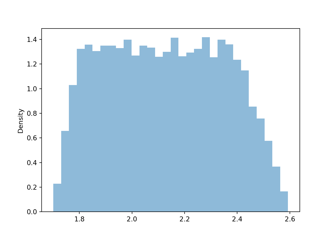
The true conditional distribution of \(Y\) given \(X=3.5\) is Uniform(1.75, 2.5). We see that the approximate distribution is a little rough at the boundaries (near 1.75 and 2.5), because of the “close to 3.5” approximation. But we would not be able to simulate the conditional distribution given \(X=3.5\) without more sophisticated methods.
10.28 Solution to Exercise 3.28
sigma = 1

X, Y = RV(Normal(0, sigma) ** 2)

R = sqrt(X ** 2 + Y ** 2)

plt.figure()
(X & Y).sim(1000).plot()
plt.show()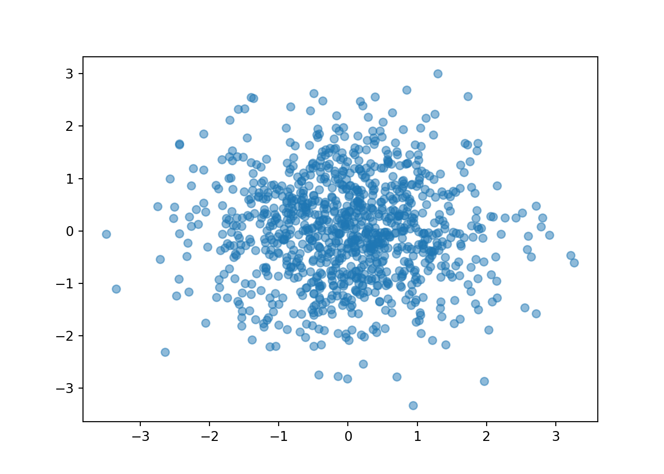
plt.figure()
R.sim(10000).plot()
plt.show()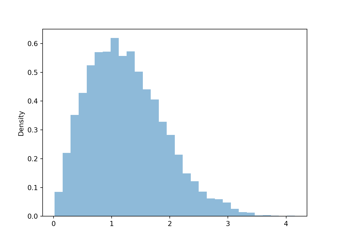
def dartboard_sim(sigma):
X, Y = RV(Normal(0, sigma) ** 2)
R = sqrt(X ** 2 + Y ** 2)
r = R.sim(10000)
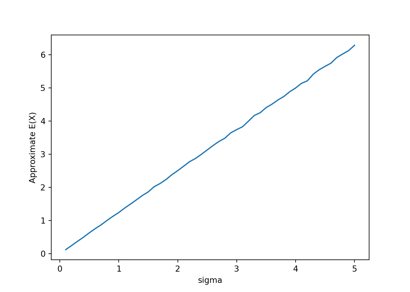
return r.count_lt(1) / r.count(), r.count_gt(12) / r.count(), r.mean()sigmas = np.arange(0.1, 5.1, 0.1)
results = np.array([dartboard_sim(sigma) for sigma in sigmas])
plt.figure()
plt.plot(sigmas, results[:, 0])
plt.xlabel('sigma')
plt.ylabel('Approximate P(X < 1)')
plt.show()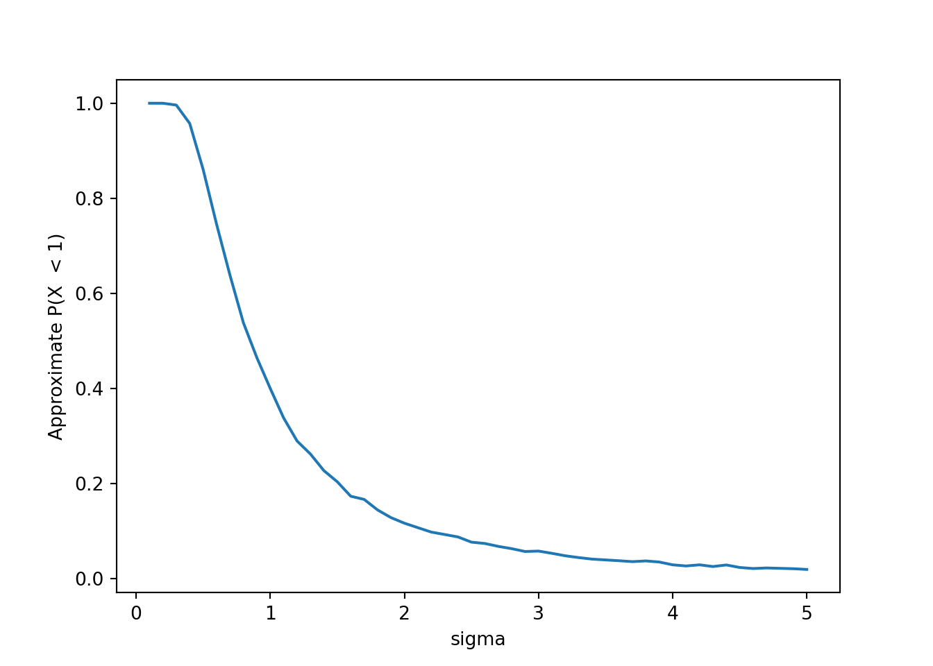
plt.figure()
plt.plot(sigmas, results[:, 1])
plt.xlabel('sigma')
plt.ylabel('Approximate P(X  > 12)')
plt.show()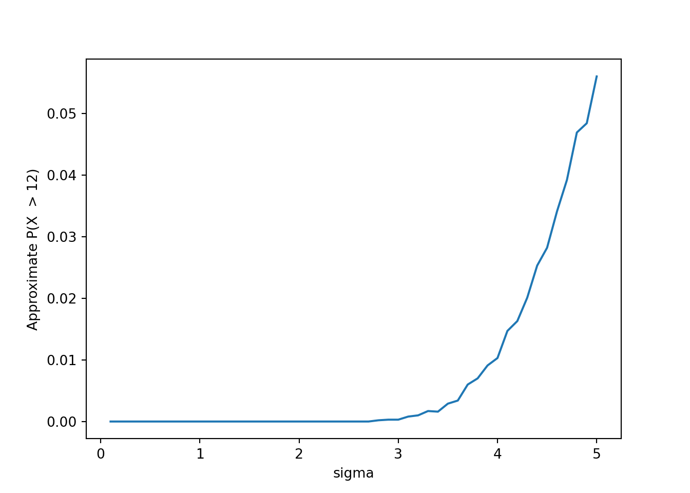
plt.figure()
plt.plot(sigmas, results[:, 2])
plt.xlabel('sigma')
plt.ylabel('Approximate E(X)')
plt.show()